- 2. Setting up the problem
- 3. Color Selection
- 4. Color Selection Code Example
- 5. 练习: Color Selection
- 6. Region Masking
- Fit lines (y=Ax+B) to identify the 3 sided region of interest
- np.polyfit() returns the coefficients [A, B] of the fit
- Color pixels red which are inside the region of interest
- Display the image
- 8. 练习:Color Region
- 9. Finding Lines of Any Color
- 11. Canny Edge Detection
- 12. Canny to Detect Lane Lines
- 13. 练习:Canny Edges
- 14. Hough Transform 霍夫变换
- 15. Hough Transform to Find Lane Lines
- 16. 练习:Hough Transform
本节要完成的工作如下:
- color selection
- region of interest selection
- grayscaling
- Gaussian smoothing
- Canny Edge Detection
- Hough Tranform line detection
2. Setting up the problem
Finding lane lines in the road:
- write code to identify and track the position of the lane lines in a series of images
- use image analysis techniques to do exactly that
3. Color Selection
What color is pure white in our combined red + green + blue [R, G, B] image?
[255,255,255]
4. Color Selection Code Example
4.1 读数据
import matplotlib.pyplot as plt
import matplotlib.image as mpimg
import numpy as np

image = mpimg.imread("test.jpg")
print('This image is: ',type(image),
         'with dimensions:', image.shape)
输出为:This image is: <class 'numpy.ndarray'> with dimensions: (720, 1280, 3)
这个image是个三维数组,在高720,宽1280的图片上,有RGB三个通道的值。
注意:第一维是长度720.
4.2 复制另一个图片数据
# Grab the x and y size and make a copy of the image
ysize = image.shape[0]
xsize = image.shape[1]
# Note: always make a copy rather than simply using "="
color_select = np.copy(image)
print("X size:",image.shape[1],"Y Size:",image.shape[0])
输出为: X size: 960 Y Size: 540
NOTE: Always make a copy of arrays or other variables in Python(color_select = np.copy(image)). If instead, you say “a = b” then all changes you make to “a” will be reflected in “b” as well!
4.3 定义RGB阈值
这个用于过滤颜色的RGB阈值,下面的例子是用于找出白色的车道线,白色的RGB值为255,255,255,取近似的230作为阈值进行判断。
# Define our color selection criteria
# Note: if you run this code, you'll find these are not sensible values!!
# But you'll get a chance to play with them soon in a quiz
red_threshold = 230
green_threshold = 230
blue_threshold = 230
rgb_threshold = [red_threshold, green_threshold, blue_threshold]
4.4 根据阈值过滤颜色的处理
# Identify pixels below the threshold
thresholds = (image[:,:,0] < rgb_threshold[0]) \
            | (image[:,:,1] < rgb_threshold[1]) \
            | (image[:,:,2] < rgb_threshold[2])
color_select[thresholds] = [0,0,0]  #
- image[:,:,0],表示整个图片上R通道的值,其shape输出为
(540, 960) - image[:,:,0] < rgb_threshold[0],即表示图片上R通道的值,是否小于其阈值,是则TRUE,否则FALSE。
- thresholds,将三个RGB比较后的值取或,即只要一个通道的值小于阈值,即满足判断条件,则为TRUE,其形状为
(540, 960),输出结果类似如下:
[[ True  True  True ...,  True  True  True]
 [ True  True  True ...,  True  True  True]
 [ True  True  True ...,  True  True  True]
 ...,
 [ True  True  True ...,  True  True  True]
 [ True  True  True ...,  True  True  True]
 [ True  True  True ...,  True  True  True]]
- color_select[thresholds] = [0,0,0],将满足条件位置的像素,设置为[0,0,0]即黑色。
4.5 图形显示
# Display the image
plt.imshow(color_select)
plt.show()

5. 练习: Color Selection
将上一节的代码串联起来,组合后如下:
import matplotlib.pyplot as plt
import matplotlib.image as mpimg
import numpy as np

# Read in the image
image = mpimg.imread('test.jpg')

# Grab the x and y size and make a copy of the image
ysize = image.shape[0]
xsize = image.shape[1]
color_select = np.copy(image)

# Define color selection criteria
###### MODIFY THESE VARIABLES TO MAKE YOUR COLOR SELECTION
red_threshold = 200
green_threshold = 200
blue_threshold = 200
######

rgb_threshold = [red_threshold, green_threshold, blue_threshold]

# Do a boolean or with the "|" character to identify
# pixels below the thresholds
thresholds = (image[:,:,0] < rgb_threshold[0]) \
            | (image[:,:,1] < rgb_threshold[1]) \
            | (image[:,:,2] < rgb_threshold[2])
color_select[thresholds] = [0,0,0]

# Display the image
plt.imshow(color_select)

# Uncomment the following code if you are running the code locally and wish to save the image
# mpimg.imsave("test-after.png", color_select)
plt.show()
输出结果如下:

6. Region Masking
The variables left_bottom, right_bottom, and apex represent the vertices of a triangular region that I would like to retain for my color selection, while masking everything else out.
上面通过RGB像素值选取了特定的颜色,获取到了车线信息,但是也同时获取到了其他白色的非车线信息,这时需要将感兴趣的区域固定在一个区域内,这样能排除车线外的物体。
左上角是y轴0点, 左下角是x轴0点
6.1 导入并复制图片数据
import matplotlib.pyplot as plt
import matplotlib.image as mpimg
import numpy as np

# Read in the image and print some stats
image = mpimg.imread('test.jpg')
print('This image is: ', type(image),
         'with dimensions:', image.shape)

# Pull out the x and y sizes and make a copy of the image
ysize = image.shape[0]
xsize = image.shape[1]
region_select = np.copy(image)
6.2 设置感兴趣区域
# Define a triangle region of interest
# Keep in mind the origin (x=0, y=0) is in the upper left in image processing
# Note: if you run this code, you'll find these are not sensible values!!
# But you'll get a chance to play with them soon in a quiz
left_bottom = [0, 539]
right_bottom = [900, 300]
apex = [400, 0]

# Fit lines (y=Ax+B) to identify the  3 sided region of interest
# np.polyfit() returns the coefficients [A, B] of the fit
fit_left = np.polyfit((left_bottom[0], apex[0]), (left_bottom[1], apex[1]), 1)
fit_right = np.polyfit((right_bottom[0], apex[0]), (right_bottom[1], apex[1]), 1)
fit_bottom = np.polyfit((left_bottom[0], right_bottom[0]), (left_bottom[1], right_bottom[1]), 1)
6.3 绘制图形
# Color pixels red which are inside the region of interest
region_select[region_thresholds] = [255, 0, 0]

# Display the image
plt.imshow(region_select)

# uncomment if plot does not display
plt.show()
绘制后图形如下,可以看到(x,y)=(0,0)在左上角:

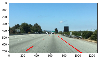
如果将坐标修改为:
left_bottom = [180, 720]
right_bottom = [1100, 720]
apex = [700, 400]
绘制的图形如下:

6.4 代码解读
- 返回斜线的A/B系数
```python
Fit lines (y=Ax+B) to identify the 3 sided region of interest
np.polyfit() returns the coefficients [A, B] of the fit
fit_left = np.polyfit((left_bottom[0], apex[0]), (left_bottom[1], apex[1]), 1) fit_right = np.polyfit((right_bottom[0], apex[0]), (right_bottom[1], apex[1]), 1) fit_bottom = np.polyfit((left_bottom[0], right_bottom[0]), (left_bottom[1], right_bottom[1]), 1)
print(fit_left) # 三角形左边的斜率 print(fit_right) # 右边的斜率 print(fit_bottom) # 底边的斜率
输出结果为,可以看出底边是斜率为0的水平直线:

```python
[-6.15384615e-01  8.30769231e+02]
[   0.8 -160. ]
[  0. 720.]
- 生成与图片相同长宽的矩形
#XX, YY = np.meshgrid(np.arange(0, xsize), np.arange(0, ysize))
XX, YY = np.meshgrid(np.arange(0, 3), np.arange(0, 4))
print(XX)
print("---")
print(YY)
输出结果如下:
- 可以看出XX,即在X方向上的值,水平方向增加,垂直方向上相同;YY正好相反。
- 而且X和Y的增长方向,零点位置,也与上面图片的坐标系吻合。
- 将XX和YY组合起来,就是矩形中各点,在特定坐标系上的坐标,比如(0,0),(1,0),(2,0)…,是矩形顶边上,从左到右的坐标值。
[[0 1 2]
 [0 1 2]
 [0 1 2]
 [0 1 2]]
---
[[0 0 0]
 [1 1 1]
 [2 2 2]
 [3 3 3]]
- 根据三角形三边的斜率参数判断
这里思考下是如何判断的?
如下图,
- 三角形的三边的YY值,分别是计算后的结果,如XX*fit_left[0] + fit_left[1]等。
- 比较矩形点与三角形三边YY值的大小,如果YY值小于左边和右边,但是大于底边,则证明在三角形之内。

region_thresholds = (YY > (XX*fit_left[0] + fit_left[1])) & \
                    (YY > (XX*fit_right[0] + fit_right[1])) & \
                    (YY < (XX*fit_bottom[0] + fit_bottom[1]))

print(region_thresholds)
输出结果(下面的结果是判断34的矩形像素,每个像素是否在指定的三角形内,显然这个右上角的34矩形,不在红色三角形内):
[[False False False]
 [False False False]
 [False False False]
 [False False False]]
- 给指定区域涂色
```python
Color pixels red which are inside the region of interest
region_select[region_thresholds] = [255, 0, 0]
Display the image
plt.imshow(region_select)
输出上面带红色三角形的图片,即将region_select像素矩阵中,指定位置的像素值,修改为红色[255,0,0].
# 7. Color and Region Combined
Next, let's combine the mask and color selection to pull only the lane lines out of the image.
Here we’re doing both the color and region selection steps, requiring that a pixel meet both the mask and color selection requirements to be retained.
本节中结合了上面的color selection和Region Selection,输出图片如下:
**代码如下:**
```python
import matplotlib.pyplot as plt
import matplotlib.image as mpimg
import numpy as np
# Read in the image
image = mpimg.imread('test.jpg')
# Grab the x and y sizes and make two copies of the image
# With one copy we'll extract only the pixels that meet our selection,
# then we'll paint those pixels red in the original image to see our selection
# overlaid on the original.
ysize = image.shape[0]
xsize = image.shape[1]
color_select= np.copy(image)
line_image = np.copy(image)
# Define our color criteria
red_threshold = 200
green_threshold = 200
blue_threshold = 200
rgb_threshold = [red_threshold, green_threshold, blue_threshold]
# Define a triangle region of interest (Note: if you run this code,
# Keep in mind the origin (x=0, y=0) is in the upper left in image processing
# you'll find these are not sensible values!!
# But you'll get a chance to play with them soon in a quiz ;)
left_bottom = [190, 720]
right_bottom = [1080, 720]
apex = [700, 400]
fit_left = np.polyfit((left_bottom[0], apex[0]), (left_bottom[1], apex[1]), 1)
fit_right = np.polyfit((right_bottom[0], apex[0]), (right_bottom[1], apex[1]), 1)
fit_bottom = np.polyfit((left_bottom[0], right_bottom[0]), (left_bottom[1], right_bottom[1]), 1)
# Mask pixels below the threshold
color_thresholds = (image[:,:,0] < rgb_threshold[0]) | \
(image[:,:,1] < rgb_threshold[1]) | \
(image[:,:,2] < rgb_threshold[2])
# Find the region inside the lines
XX, YY = np.meshgrid(np.arange(0, xsize), np.arange(0, ysize))
region_thresholds = (YY > (XX*fit_left[0] + fit_left[1])) & \
(YY > (XX*fit_right[0] + fit_right[1])) & \
(YY < (XX*fit_bottom[0] + fit_bottom[1]))
# Mask color selection
color_select[color_thresholds] = [0,0,0]
# Find where image is both colored right and in the region
line_image[~color_thresholds & region_thresholds] = [255,0,0]
# Display our two output images
plt.imshow(color_select)
plt.imshow(line_image)
# uncomment if plot does not display
# plt.show()
7.1 代码解读
本部分代码是上面5和6的结合,步骤如下:
- 读取图片。
- 复制图片副本。
- 设定用于过滤颜色的RGB阈值,白色的话,这里设置为[200,200,200]。
- 设定限定区域顶点左边,这是是一个三角形。
- 判断图片上的RGB值,与指定RGB阈值的大小,得到一组BOOL值的矩阵。(该BOOL矩阵表示,如果是白色则为FALSE)
- 判断图片矩形的坐标值,与上面限定区域值的大小,得到一组BOOL值的矩阵。(该BOOL矩阵表示,如果在三角形内部则为TRUE)
- 针对指定矩形,进行RGB值得处理。
- 显示两幅图形。
- 针对指定矩形,进行RGB值处理
- 处理[color_select],将非白色的区域,全部设置为黑色[0,0,0]。
- 处理[line_image],使用
~color_thresholds,选定白色区域,用& region_thresholds与上三角形的区域,结果为三角形内的白色区域,将其设置为红色[255,0,0]。
# Mask color selection
color_select[color_thresholds] = [0,0,0]
# Find where image is both colored right and in the region
line_image[~color_thresholds & region_thresholds] = [255,0,0]
- 显示上面处理后的color_select和line_image。
# Display our two output images
plt.imshow(color_select)
plt.imshow(line_image)
8. 练习:Color Region
融合上面的代码,输出如下的图形:

import matplotlib.pyplot as plt
import matplotlib.image as mpimg
import numpy as np

# Read in the image
image = mpimg.imread('test.jpg')

# Grab the x and y size and make a copy of the image
ysize = image.shape[0]
xsize = image.shape[1]
color_select = np.copy(image)
line_image = np.copy(image)

# Define color selection criteria
# MODIFY THESE VARIABLES TO MAKE YOUR COLOR SELECTION
red_threshold = 200
green_threshold = 200
blue_threshold = 200

rgb_threshold = [red_threshold, green_threshold, blue_threshold]

# Define the vertices of a triangular mask.
# Keep in mind the origin (x=0, y=0) is in the upper left
# MODIFY THESE VALUES TO ISOLATE THE REGION
# WHERE THE LANE LINES ARE IN THE IMAGE

left_bottom = [190, 720]
right_bottom = [1060, 720]
apex = [650, 400]

# Perform a linear fit (y=Ax+B) to each of the three sides of the triangle
# np.polyfit returns the coefficients [A, B] of the fit
fit_left = np.polyfit((left_bottom[0], apex[0]), (left_bottom[1], apex[1]), 1)
fit_right = np.polyfit((right_bottom[0], apex[0]), (right_bottom[1], apex[1]), 1)
fit_bottom = np.polyfit((left_bottom[0], right_bottom[0]), (left_bottom[1], right_bottom[1]), 1)

# Mask pixels below the threshold
color_thresholds = (image[:,:,0] < rgb_threshold[0]) | \
                    (image[:,:,1] < rgb_threshold[1]) | \
                    (image[:,:,2] < rgb_threshold[2])

# Find the region inside the lines
XX, YY = np.meshgrid(np.arange(0, xsize), np.arange(0, ysize))
region_thresholds = (YY > (XX*fit_left[0] + fit_left[1])) & \
                    (YY > (XX*fit_right[0] + fit_right[1])) & \
                    (YY < (XX*fit_bottom[0] + fit_bottom[1]))

# Mask color and region selection
color_select[color_thresholds | ~region_thresholds] = [0, 0, 0]
# Color pixels red where both color and region selections met
line_image[~color_thresholds & region_thresholds] = [255, 0, 0]

# Display the image and show region and color selections
plt.imshow(image)
x = [left_bottom[0], right_bottom[0], apex[0], left_bottom[0]]
y = [left_bottom[1], right_bottom[1], apex[1], left_bottom[1]]
plt.plot(x, y, 'b--', lw=4)
plt.imshow(color_select)
plt.imshow(line_image)
plt.show()
8.1 代码解读
从最开始的图片读取,到后面的得到颜色阈值与三角形区域内BOOL值矩阵,处理代码都是一样的,但是最后两步有细微差异。
- 针对矩阵进行颜色处理
~region_thresholds指非三角形区域,color_thresholds指非白色区域,结果就是将三角形以外区域,以及非白色区域(三角形内),处理成黑色。
~color_thresholds指白色的区域,region_thresholds指三角形内,即将三角形内的白色区域变成红色。

# Mask color and region selection
color_select[color_thresholds | ~region_thresholds] = [0, 0, 0]
# Color pixels red where both color and region selections met
line_image[~color_thresholds & region_thresholds] = [255, 0, 0]
- 图形显示处理
这里画了一个连续的图形,x和y分别表示连续图形各个顶点的x和y坐标,这里是[左下角,右下角,顶点,左下角]这样构成一个封闭的图形。最后用plt.plot()画出来。
# Display the image and show region and color selections
plt.imshow(image)
x = [left_bottom[0], right_bottom[0], apex[0], left_bottom[0]]
y = [left_bottom[1], right_bottom[1], apex[1], left_bottom[1]]
plt.plot(x, y, 'b--', lw=4)
plt.imshow(color_select)
plt.imshow(line_image)
plt.show()
显示的图形如下:

9. Finding Lines of Any Color
上面通过color和region的selection,选取了车道线lane,但是并不是所有时候车道线都是白色,另外随着天气等外界因素,颜色也可能会改变。 下面将学习更通用的方式去检测任何颜色的lane。
As it happens, lane lines are not always the same color, and even lines of the same color under different lighting conditions (day, night, etc) may fail to be detected by our simple color selection.
What we need is to take our algorithm to the next level to detect lines of any color using sophisticated computer vision methods.
关于下一部分要用到的ComputerVision,可以学习这个课程introduction-to-computer-vision.
11. Canny Edge Detection
With edge detection, the goal is to identify the boundaries of an object in an image. To do this,
- convert to grayscale, 转成灰度图像
- compute the gradient, 计算其梯度
- 通过寻找最大梯度找到边界
edges = cv2.Canny(gray,low_threshold,high_threshold)
- gray表示灰度图像,edges表示处理后输出的边界
- threshold表示边界检测强度
12. Canny to Detect Lane Lines
12.1 灰度变换和edge检测
import matplotlib.pyplot as plt
import matplotlib.image as mpimg
image = mpimg.imread('exit-ramp.jpg')
plt.imshow(image)

import cv2  #bringing in OpenCV libraries
# 灰度变换
gray = cv2.cvtColor(image, cv2.COLOR_RGB2GRAY) #grayscale conversion
plt.imshow(gray, cmap='gray')

# 边缘检测
edges = cv2.Canny(gray, low_threshold, high_threshold)
plt.imshow(edges)
- The algorithm will first detect strong edge (strong gradient) pixels above the high_threshold, and reject pixels below the low_threshold.
- Next, pixels with values between the low_threshold and high_threshold will be included as long as they are connected to strong edges.
输出后图形如下:

12.2 代码解读
#doing all the relevant imports
import matplotlib.pyplot as plt
import matplotlib.image as mpimg
import numpy as np
import cv2

# Read in the image and convert to grayscale
image = mpimg.imread('exit-ramp.jpg')
gray = cv2.cvtColor(image, cv2.COLOR_RGB2GRAY)

# Define a kernel size for Gaussian smoothing / blurring
# Note: this step is optional as cv2.Canny() applies a 5x5 Gaussian internally
kernel_size = 3
blur_gray = cv2.GaussianBlur(gray,(kernel_size, kernel_size), 0)

# Define parameters for Canny and run it
# NOTE: if you try running this code you might want to change these!
low_threshold = 10
high_threshold = 100
edges = cv2.Canny(blur_gray, low_threshold, high_threshold)

# Display the image
plt.imshow(edges, cmap='Greys_r')
输出图形如下:

- 如何设定low_threshold和high_threshold
This range implies that derivatives (essentially, the value differences from pixel to pixel) will be on the scale of tens or hundreds. 这个用于表示RGB变化的范围大小,一般两者之间是1:2或1:3的关系。 如果设置为如下很小的值,将会导致大量边界被检测出来,如下:
low_threshold = 1
high_threshold = 10
edges = cv2.Canny(blur_gray, low_threshold, high_threshold)

- GaussianBlur函数,用于平滑除燥
We’ll also include Gaussian smoothing, before running Canny, which is essentially a way of suppressing noise and spurious gradients by averaging (check out the OpenCV docs for GaussianBlur).
- cv2.Canny() actually applies Gaussian smoothing internally。
- You can choose the kernel_size for Gaussian smoothing to be any odd number. A larger kernel_size implies averaging, or smoothing, over a larger area. The example in the previous lesson was kernel_size = 3.
13. 练习:Canny Edges
需要调整threshold和kernelsize参数,得到一个理想的边界图像,但是为什么要这么调整,各种原理没有掌握!!
# Do all the relevant imports
import matplotlib.pyplot as plt
import matplotlib.image as mpimg
import numpy as np
import cv2

# Read in the image and convert to grayscale
# Note: in the previous example we were reading a .jpg
# Here we read a .png and convert to 0,255 bytescale
image = mpimg.imread('exit-ramp.jpg')
gray = cv2.cvtColor(image,cv2.COLOR_RGB2GRAY)

# Define a kernel size for Gaussian smoothing / blurring
kernel_size = 5 # Must be an odd number (3, 5, 7...)
blur_gray = cv2.GaussianBlur(gray,(kernel_size, kernel_size),0)

# Define our parameters for Canny and run it
low_threshold = 80
high_threshold = 200
edges = cv2.Canny(blur_gray, low_threshold, high_threshold)

# Display the image
plt.imshow(edges, cmap='Greys_r')

14. Hough Transform 霍夫变换
14.1 霍夫空间介绍
霍夫变换就是将一般的图片空间,转换成霍夫Hough空间。如下图中,函数y=mx+b,在霍夫空间上对应一个点,因为直线斜率固定,所以m为定值,直线位置固定,所以b为定值。

- image space 的一条固定的线段,在Hough Space中是一个点。
- 反之,一个image space中的点,在Hough Space中是一条线段,表示有很多不同斜率m和位置b的线段可以通过该点。

下图说明,x1和x2两点,可以连接成一条直线,故能有相同的m和b,那么反映在hough空间上,说明两个直线有交点。

14.2 寻找直线
寻找图像空间直线的策略,就是寻找霍夫空间中线的交点。

- 图像空间的一个点,在霍夫空间是一条直线
- 如果霍夫空间的直线,都相交于某个点(m0,b0),说明图像空间的点能够连接成一条直线y=m0*x + b
为了实现上面的,
- 运行canny算法,找到图像中所有位于边缘的点,这些点在霍夫空间中是一条直线。
- 如果在霍夫空间找到一个有多条交叉的位置,则说明图像空间中的点位于一条直线上。
- 极坐标中重新定义直线

比如上面一条图片空间的直线xcosθ + ysinθ = P,在霍夫空间中是一个点,原理相同。
反之,如果是多个点,在霍夫空间表现成多个正弦曲线,并且有交点:

15. Hough Transform to Find Lane Lines
通过函数HoughLinesP获取图像边界。
lines = cv2.HoughLinesP(masked_edges, rho, theta, threshold, np.array([]),min_line_length, max_line_gap)
- masked_edges,是上面的canny函数检测出来的边界图形。
- lines,即函数的输出,是一系列线段。
- rho和theta,表示霍夫空间中网格grid的像素数和半径。In Hough space, we have a grid laid out along the (Θ, ρ) axis. You need to specify rho in units of pixels and theta in units of radians.
- rho takes a minimum value of 1, and a reasonable starting place for theta is 1 degree (pi/180 in radians).
- threshold,表示如果要能判断为图片空间是一段直线的话,在一个grid内的最小相交数。
- np.array([]),is just a placeholder, no need to change it.
- min_line_length,要能判断为一条直线,其最小的长度(像素数)
- max_line_gap,两个线段之间,超过多远(像素),就不能连接起来了。
15.1 代码
# Do relevant imports
import matplotlib.pyplot as plt
import matplotlib.image as mpimg
import numpy as np
import cv2

# Read in and grayscale the image
image = mpimg.imread('exit-ramp.jpg')
gray = cv2.cvtColor(image,cv2.COLOR_RGB2GRAY)

# Define a kernel size and apply Gaussian smoothing
kernel_size = 5
blur_gray = cv2.GaussianBlur(gray,(kernel_size, kernel_size),0)

# Define our parameters for Canny and apply
low_threshold = 50
high_threshold = 150
masked_edges = cv2.Canny(blur_gray, low_threshold, high_threshold)

# Define the Hough transform parameters
# Make a blank the same size as our image to draw on
rho = 1
theta = np.pi/180
threshold = 5
min_line_length = 50
max_line_gap = 1
line_image = np.copy(image)*0 #creating a blank to draw lines on

# Run Hough on edge detected image
lines = cv2.HoughLinesP(masked_edges, rho, theta, threshold, np.array([]),
                            min_line_length, max_line_gap)

# Iterate over the output "lines" and draw lines on the blank
for line in lines:
    for x1,y1,x2,y2 in line:
        cv2.line(line_image,(x1,y1),(x2,y2),(255,0,0),10)

# Create a "color" binary image to combine with line image
color_edges = np.dstack((masked_edges, masked_edges, masked_edges))

# Draw the lines on the edge image
combo = cv2.addWeighted(color_edges, 0.8, line_image, 1, 0)
plt.imshow(combo)
图像输出为:

15.2 代码解读
上面的处理步骤如下:
- 读取图片,并进行灰度变换。
- 进行GaussianBlur平滑处理。
- 使用Canny进行边界检测处理。
- 使用HoughLinesP,将各个零散的边界,复合条件的连接起来,并输出为lines。
- 使用for循环lines上的点,生成红色的线条line_image。
- 生成黑色背景白色线条的底图color_edges。
- 使用addWeighted,将上面的line_image和color_edges叠加显示。
- line_image图

- color_edges图

16. 练习:Hough Transform
生成图:

import matplotlib.pyplot as plt
import matplotlib.image as mpimg
import numpy as np
import cv2


# Read in and grayscale the image
image = mpimg.imread('exit-ramp.jpg')
gray = cv2.cvtColor(image,cv2.COLOR_RGB2GRAY)

# Define a kernel size and apply Gaussian smoothing
kernel_size = 5
blur_gray = cv2.GaussianBlur(gray,(kernel_size, kernel_size),0)

# Define our parameters for Canny and apply
low_threshold = 100
high_threshold = 150
edges = cv2.Canny(blur_gray, low_threshold, high_threshold)

# Next we'll create a masked edges image using cv2.fillPoly()
mask = np.zeros_like(edges)
ignore_mask_color = 255

# This time we are defining a four sided polygon to mask
imshape = image.shape
#vertices = np.array([[(0,imshape[0]),(0, 0), (imshape[1], 0), (imshape[1],imshape[0])]], dtype=np.int32)
vertices = np.array([[(0,imshape[0]),((imshape[1]/2)-50, imshape[0]/2), ((imshape[1]/2)+50, imshape[0]/2), (imshape[1],imshape[0])]], dtype=np.int32)
cv2.fillPoly(mask, vertices, ignore_mask_color)
masked_edges = cv2.bitwise_and(edges, mask)

# Define the Hough transform parameters
# Make a blank the same size as our image to draw on
rho = 1 # distance resolution in pixels of the Hough grid
theta = np.pi/180 # angular resolution in radians of the Hough grid
threshold = 5     # minimum number of votes (intersections in Hough grid cell)
min_line_length = 40 #minimum number of pixels making up a line
max_line_gap = 2    # maximum gap in pixels between connectable line segments
line_image = np.copy(image)*0 # creating a blank to draw lines on

# Run Hough on edge detected image
# Output "lines" is an array containing endpoints of detected line segments
lines = cv2.HoughLinesP(masked_edges, rho, theta, threshold, np.array([]),
                            min_line_length, max_line_gap)

# Iterate over the output "lines" and draw lines on a blank image
for line in lines:
    for x1,y1,x2,y2 in line:
        cv2.line(line_image,(x1,y1),(x2,y2),(255,0,0),10)

# Create a "color" binary image to combine with line image
color_edges = np.dstack((edges, edges, edges))

# Draw the lines on the edge image
lines_edges = cv2.addWeighted(color_edges, 0.8, line_image, 1, 0)
plt.imshow(lines_edges)
本节心得,一定要弄清楚各个参数的意义,否则即使调整参数,也是漫无目的的调。
- 选取目标区域:
vertices = np.array([[(0,imshape[0]),((imshape[1]/2)-50, imshape[0]/2), ((imshape[1]/2)+50, imshape[0]/2), (imshape[1],imshape[0])]], dtype=np.int32)


16.1 代码解读
- 图片读取,灰度变换cvtColor。
- 高斯变换GaussianBlur。
- 边缘检测Canny。
- 指定区域大小,处理边界数据。
- 使用HoughLinesP,将各个零散的边界,复合条件的连接起来,并输出为lines。
- 使用for循环lines上的点,生成红色的线条line_image。
- 生成黑色背景白色线条的底图color_edges。
- 使用addWeighted,将上面的line_image和color_edges叠加显示。
指定区域大小,处理边界数据
# Next we'll create a masked edges image using cv2.fillPoly()
mask = np.zeros_like(edges)
ignore_mask_color = 255

# This time we are defining a four sided polygon to mask
imshape = image.shape
vertices = np.array([[(0,imshape[0]),((imshape[1]/2)-50, imshape[0]/2), ((imshape[1]/2)+50, imshape[0]/2), (imshape[1],imshape[0])]], dtype=np.int32)
cv2.fillPoly(mask, vertices, ignore_mask_color)
masked_edges = cv2.bitwise_and(edges, mask)
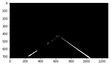
- np.zeros_like(edges),生成与edges相同的矩阵,形状为(540, 960),值都是0,如果用plt.imshow(mask)的话,就是一个黑色矩形,imshow(edges)是黑色矩形中有检测出来的边界线。
- vertices,是一个指定大小的区域,这里是一个梯形。
- cv2.fillPoly(mask, vertices, ignore_mask_color),将梯形填充到黑色矩形中,输出图形如下:

- masked_edges = cv2.bitwise_and(edges, mask),输出图形如下:

fillPoly和bitwise_and函数的用法要注意!