- 1. 项目介绍
- 2. 识别车线
- 3. helper functions介绍
- 4. 代码详细
- 4.1 Import Packages
- 4.2 Read in an Image
- 4.3 Ideas for Lane Detection Pipeline
- 4.4 Helper Functions
- 4.5 Test Images
- 4.6 Applies the Grayscale transform/gaussian_blur/Canny transform
- 4.7 Set a region
- 4.8 Run Hough on edge detected image
- 4.9 Merge Lines with the original image
- 4.10 Build a Lane Finding Pipeline
- 4.11 Test on Videos
- 98. 参考信息
1. 项目介绍
目的: identify lane lines on the road
- Your first goal is to write code including a series of steps (pipeline) that identify and draw the lane lines on a few test images.
- Once you can successfully identify the lines in an image, you can cut and paste your code into the block provided to run on a video stream.
- 处理一系列单独的图片-识别出车线并叠加红色线条,develop your pipeline on a series of individual images
- 将上述的方法应用到video中,apply the result to a video stream (really just a series of images) - 输出结果类似raw-lines-example.mp4
- 用插值的方式,将识别出来的车道线连接起来,get creative and try to average and/or extrapolate the line segments you’ve detected to map out the full extent of the lane lines - 输出结果类似P1_example.mp4
- 写一个总结文档,there is a brief writeup to complete
文件目录结构:
- writeup_template.md, 总结文档
- P1.ipynb, notebook文件
- examples文件夹,包含原始图片及处理后的图片,原始video和处理后的video
- test_images文件夹,左行右行等各种原始图片
- test_videos文件夹,三个原始的行驶video
- test_videos_output文件夹,结果输出用的文件夹
- To find the lanes I used below steps as my pipeline:
- Converting image to grayscale
- Blurring an image by a Gaussian function
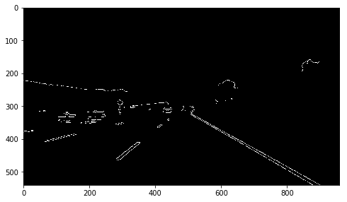
- Using CannyEdge to find the edges
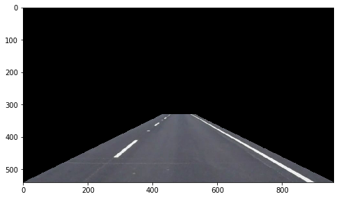
- Applying the region of interest and keep only the edges which are present in Region of Interest
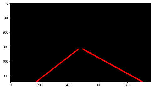
- Using hough algorithm to detect the lines from the image
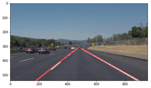
- Adding the lane lines to the original image
- About the draw_lines() function:
- Creating two groups of lines based on the slope and also exclude lines that are not in the specific threshold.
- Using the points of left and right line get the slope and b of y = slope*x + b
- Calculating start and ends points to make lines with a straight line
- Calculating the means for creating the left lane and right lane
2. 识别车线
The tools you have are:
- color selection
- region of interest selection
- grayscaling
- Gaussian smoothing
- Canny Edge Detection
- Hough Tranform line detection
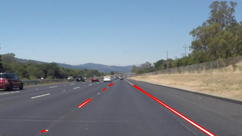
通过helper functions可以检测出车道线:
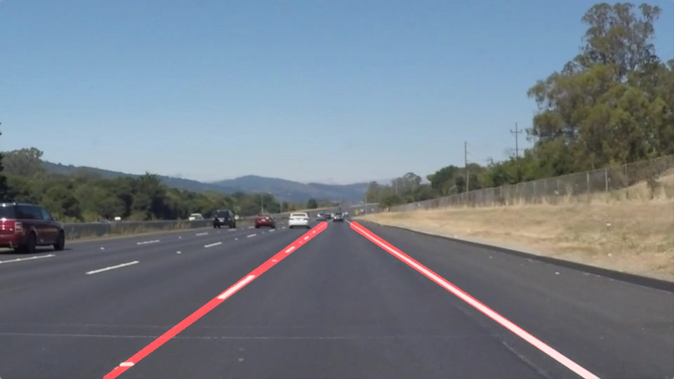
需要通过 connect/average/extrapolate 等手段将车道线处理成如下的效果:
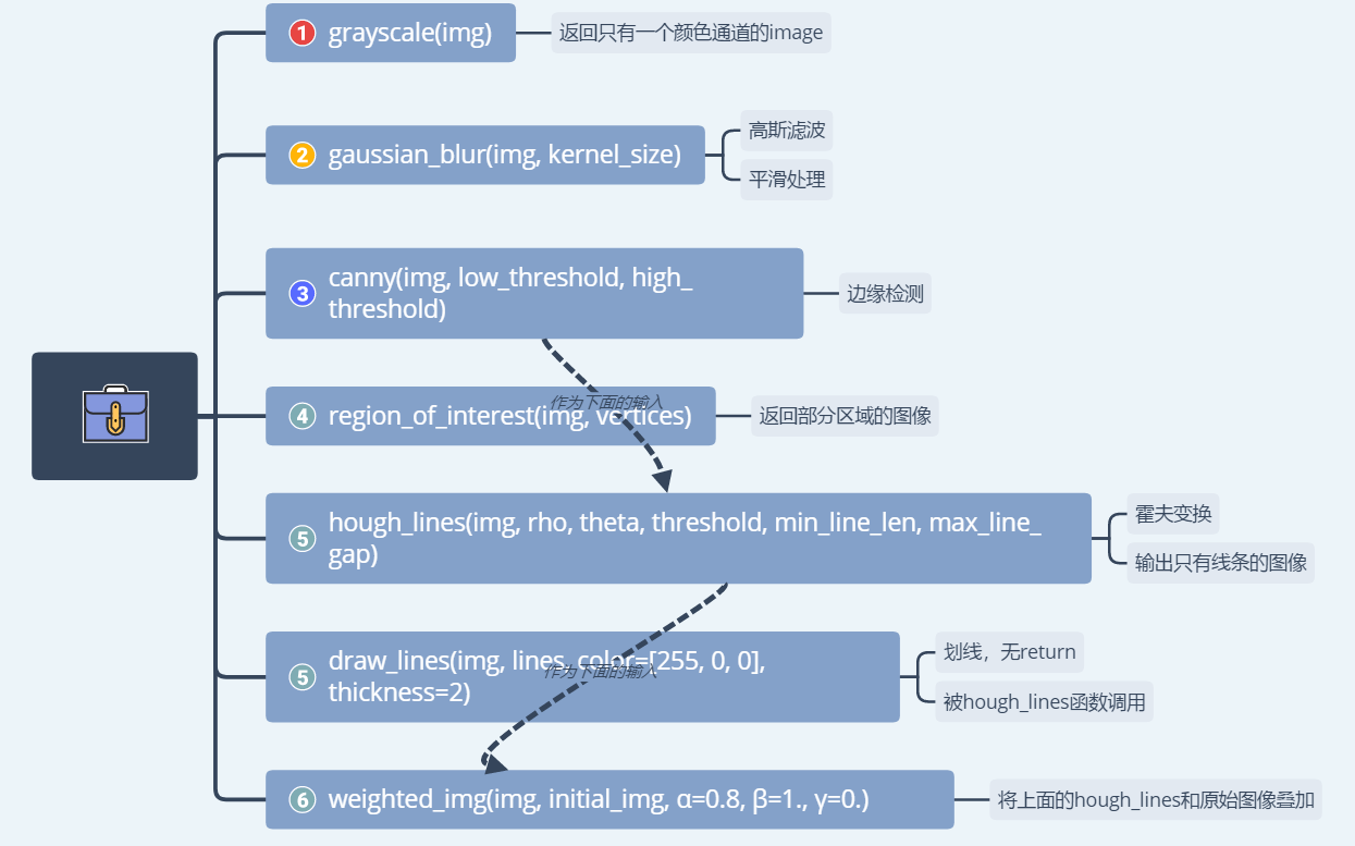
3. helper functions介绍
4. 代码详细
4.1 Import Packages
#importing some useful packages
import matplotlib.pyplot as plt
import matplotlib.image as mpimg
import numpy as np
import cv2
%matplotlib inline
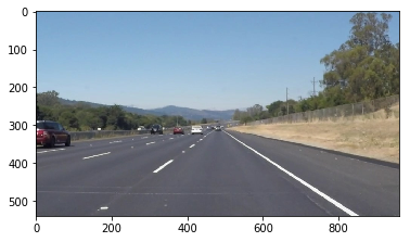
4.2 Read in an Image
#reading in an image
image = mpimg.imread('test_images/solidWhiteRight.jpg')

#printing out some stats and plotting
print('This image is:', type(image), 'with dimensions:', image.shape)
plt.imshow(image)  # if you wanted to show a single color channel image called 'gray', for example, call as plt.imshow(gray, cmap='gray')
4.3 Ideas for Lane Detection Pipeline
**Some OpenCV functions (beyond those introduced in the lesson) that might be useful for this project are:**

`cv2.inRange()` for color selection
`cv2.fillPoly()` for regions selection
`cv2.line()` to draw lines on an image given endpoints
`cv2.addWeighted()` to coadd / overlay two images
`cv2.cvtColor()` to grayscale or change color
`cv2.imwrite()` to output images to file
`cv2.bitwise_and()` to apply a mask to an image

**Check out the OpenCV documentation to learn about these and discover even more awesome functionality!**
4.4 Helper Functions
import math

def grayscale(img):
    """Applies the Grayscale transform
    This will return an image with only one color channel
    but NOTE: to see the returned image as grayscale
    (assuming your grayscaled image is called 'gray')
    you should call plt.imshow(gray, cmap='gray')"""
    #plt.imshow(gray, cmap='gray')
    return cv2.cvtColor(img, cv2.COLOR_RGB2GRAY)
    # Or use BGR2GRAY if you read an image with cv2.imread()
    # return cv2.cvtColor(img, cv2.COLOR_BGR2GRAY)

def canny(img, low_threshold, high_threshold):
    """Applies the Canny transform"""
    return cv2.Canny(img, low_threshold, high_threshold)

def gaussian_blur(img, kernel_size):
    """Applies a Gaussian Noise kernel"""
    return cv2.GaussianBlur(img, (kernel_size, kernel_size), 0)

def region_of_interest(img, vertices):
    """
    Applies an image mask.

    Only keeps the region of the image defined by the polygon
    formed from `vertices`. The rest of the image is set to black.
    `vertices` should be a numpy array of integer points.
    """
    #defining a blank mask to start with
    mask = np.zeros_like(img)

    #defining a 3 channel or 1 channel color to fill the mask with depending on the input image
    if len(img.shape) > 2:
        channel_count = img.shape[2]  # i.e. 3 or 4 depending on your image
        ignore_mask_color = (255,) * channel_count
    else:
        ignore_mask_color = 255

    #filling pixels inside the polygon defined by "vertices" with the fill color
    cv2.fillPoly(mask, vertices, ignore_mask_color)

    #returning the image only where mask pixels are nonzero
    masked_image = cv2.bitwise_and(img, mask)
    return masked_image

def draw_lines_ori(img, lines, color=[255, 0, 0], thickness=7):
    """
    NOTE: this is the function you might want to use as a starting point once you want to
    average/extrapolate the line segments you detect to map out the full
    extent of the lane (going from the result shown in raw-lines-example.mp4
    to that shown in P1_example.mp4).

    Think about things like separating line segments by their
    slope ((y2-y1)/(x2-x1)) to decide which segments are part of the left
    line vs. the right line.  Then, you can average the position of each of
    the lines and extrapolate to the top and bottom of the lane.

    This function draws `lines` with `color` and `thickness`.
    Lines are drawn on the image inplace (mutates the image).
    If you want to make the lines semi-transparent, think about combining
    this function with the weighted_img() function below
    """


    for line in lines:
        for x1,y1,x2,y2 in line:
            cv2.line(img, (x1, y1), (x2, y2), color, thickness)


def draw_lines(img, lines, color=[255, 0, 0], thickness=7):

     #list to get positives and negatives values

    x_bottom_pos = []
    x_upperr_pos = []
    x_bottom_neg = []
    x_upperr_neg = []

    y_bottom = 540
    y_upperr = 315

    slope = 0
    b = 0

    #get x upper and bottom to lines with slope positive and negative
    for line in lines:
        for x1,y1,x2,y2 in line:
            #test and filter values to slope
            if ((y2-y1)/(x2-x1)) > 0.5 and ((y2-y1)/(x2-x1)) < 0.8 :

                slope = ((y2-y1)/(x2-x1))
                b = y1 - slope*x1

                x_bottom_pos.append((y_bottom - b)/slope)
                x_upperr_pos.append((y_upperr - b)/slope)

            elif ((y2-y1)/(x2-x1)) < -0.5 and ((y2-y1)/(x2-x1)) > -0.8:

                slope = ((y2-y1)/(x2-x1))
                b = y1 - slope*x1

                x_bottom_neg.append((y_bottom - b)/slope)
                x_upperr_neg.append((y_upperr - b)/slope)

    #creating a new 2d array with means
    lines_mean = np.array([[int(np.mean(x_bottom_pos)), int(np.mean(y_bottom)), int(np.mean(x_upperr_pos)), int(np.mean(y_upperr))],
                           [int(np.mean(x_bottom_neg)), int(np.mean(y_bottom)), int(np.mean(x_upperr_neg)), int(np.mean(y_upperr))]])

    #Drawing the lines
    for i in range(len(lines_mean)):
        cv2.line(img, (lines_mean[i,0], lines_mean[i,1]), (lines_mean[i,2], lines_mean[i,3]), color, thickness)


def hough_lines(img, rho, theta, threshold, min_line_len, max_line_gap):
    """
    `img` should be the output of a Canny transform.

    Returns an image with hough lines drawn.
    """
    lines = cv2.HoughLinesP(img, rho, theta, threshold, np.array([]), minLineLength=min_line_len, maxLineGap=max_line_gap)
    line_img = np.zeros((img.shape[0], img.shape[1], 3), dtype=np.uint8)
    draw_lines(line_img, lines)
    return line_img

# Python 3 has support for cool math symbols.

def weighted_img(img, initial_img, α=0.8, β=1., γ=0.):
    """
    `img` is the output of the hough_lines(), An image with lines drawn on it.
    Should be a blank image (all black) with lines drawn on it.

    `initial_img` should be the image before any processing.

    The result image is computed as follows:

    initial_img * α + img * β + γ
    NOTE: initial_img and img must be the same shape!
    """
    return cv2.addWeighted(initial_img, α, img, β, γ)
4.5 Test Images
Build your pipeline to work on the images in the directory “test_images”
You should make sure your pipeline works well on these images before you try the videos.
import os
imgpath = os.listdir("test_images/")
print(imgpath)
4.6 Applies the Grayscale transform/gaussian_blur/Canny transform
image = mpimg.imread('test_images/solidWhiteCurve.jpg')
color_select = np.copy(image)

# gray transform
gray = grayscale(color_select)

# Define a kernel size for Gaussian smoothing / blurring
kernel_size = 5
blur_gray = gaussian_blur(gray,kernel_size)

# Define parameters for Canny and run it
low_threshold = 100
high_threshold = 250
edges = canny(blur_gray, low_threshold, high_threshold)

# Display the image
plt.figure(figsize=(8,6))
plt.imshow(edges, cmap='Greys_r')
4.7 Set a region
# This time we are defining a four sided polygon to mask
imshape = image.shape
left_bottom = (0,imshape[0]) # 1
right_bottom = (imshape[1],imshape[0]) # 4
right_top =  ((imshape[1]/2)+50, (imshape[0]/2 + 60)) # 3
left_top = ((imshape[1]/2 )-50, (imshape[0]/2 + 60)) # 2

vertices = np.array([[left_bottom,left_top,right_top, right_bottom]], dtype=np.int32)
selectimg = region_of_interest(color_select,vertices)

plt.figure(figsize=(8,6))
plt.imshow(selectimg)
selectedges = region_of_interest(edges,vertices)

plt.figure(figsize=(8,6))
plt.imshow(selectedges, cmap='Greys_r')

4.8 Run Hough on edge detected image
rho = 1
theta = np.pi/90
threshold = 30
min_line_length = 40
max_line_gap = 400

lines = hough_lines(selectedges, rho, theta, threshold,min_line_length, max_line_gap)

plt.figure(figsize=(8,6))
plt.imshow(lines)
4.9 Merge Lines with the original image
lines_edges = weighted_img(lines, image, α=0.8, β=1., γ=0.)

plt.figure(figsize=(8,6))
plt.imshow(lines_edges)
4.10 Build a Lane Finding Pipeline
Build the pipeline
def pipeline_img(image,
                   kernel_size = 5,
                   low_threshold = 100, high_threshold=250,
                   rho=1, theta=np.pi/90, threshold=30,
                   min_line_len=40, max_line_gap=400):

    color_select = np.copy(image)

    # gray transform
    gray = grayscale(color_select)

    # Gaussian smoothing / blurring
    blur_gray = gaussian_blur(gray, kernel_size)

    #finding edges
    edges = canny(blur_gray, low_threshold, high_threshold)

    #setting vertices
    imshape = image.shape
    left_bottom = (0,imshape[0]) # 1
    right_bottom = (imshape[1],imshape[0]) # 4
    right_top =  ((imshape[1]/2)+50, (imshape[0]/2 + 60)) # 3
    left_top = ((imshape[1]/2 )-50, (imshape[0]/2 + 60)) # 2

    vertices = np.array([[left_bottom,left_top,right_top, right_bottom]], dtype=np.int32)

    #creating a region of interest
    masked_edges = region_of_interest(edges, vertices)

    #finding lines
    lines = hough_lines(masked_edges, rho, theta, threshold, min_line_len, max_line_gap)

    #merge with original image
    lines_edges = weighted_img(lines, image, α=0.8, β=1., γ=0.)

    return lines_edges
** Processing the images and saving them to the ouput**
import os
imgname = os.listdir("test_images/")

for img in imgname:
    imgpath = "test_images/" + img
    image = mpimg.imread(imgpath)

    image_processed = pipeline_img(image,
                   kernel_size = 5,
                   low_threshold = 100, high_threshold=250,
                   rho=1, theta=np.pi/90, threshold=30,
                   min_line_len=40, max_line_gap=400)
    mpimg.imsave("test_images_output/" + img, image_processed)
4.11 Test on Videos
# Import everything needed to edit/save/watch video clips

from moviepy.editor import VideoFileClip
from IPython.display import HTML

def process_image(image):
    # NOTE: The output you return should be a color image (3 channel) for processing video below
    # TODO: put your pipeline here,
    # you should return the final output (image where lines are drawn on lanes)

    result = pipeline_img(image,
                    kernel_size = 5,
                   low_threshold = 100, high_threshold=250,
                   rho=1, theta=np.pi/90, threshold=30,
                   min_line_len=40, max_line_gap=400)

    return result

white_output = 'test_videos_output/solidWhiteRight.mp4'
## To speed up the testing process you may want to try your pipeline on a shorter subclip of the video
## To do so add .subclip(start_second,end_second) to the end of the line below
## Where start_second and end_second are integer values representing the start and end of the subclip
## You may also uncomment the following line for a subclip of the first 5 seconds
##clip1 = VideoFileClip("test_videos/solidWhiteRight.mp4").subclip(0,5)
clip1 = VideoFileClip("test_videos/solidWhiteRight.mp4")
white_clip = clip1.fl_image(process_image) #NOTE: this function expects color images!!
%time white_clip.write_videofile(white_output, audio=False)
HTML("""
<video width="960" height="540" controls>
  <source src="{0}">
</video>
""".format(white_output))
yellow_output = 'test_videos_output/solidYellowLeft.mp4'
## To speed up the testing process you may want to try your pipeline on a shorter subclip of the video
## To do so add .subclip(start_second,end_second) to the end of the line below
## Where start_second and end_second are integer values representing the start and end of the subclip
## You may also uncomment the following line for a subclip of the first 5 seconds
##clip2 = VideoFileClip('test_videos/solidYellowLeft.mp4').subclip(0,5)
clip2 = VideoFileClip('test_videos/solidYellowLeft.mp4')
yellow_clip = clip2.fl_image(process_image)
%time yellow_clip.write_videofile(yellow_output, audio=False)
def draw_lines2(img, lines, color=[255, 0, 0], thickness=7):

     #list to get positives and negatives values

    x_bottom_pos = []
    x_upperr_pos = []
    x_bottom_neg = []
    x_upperr_neg = []

    y_bottom = 720
    y_upperr = 450

    slope = 0
    b = 0

    #get x upper and bottom to lines with slope positive and negative
    for line in lines:
        for x1,y1,x2,y2 in line:
            #test and filter values to slope
            if ((y2-y1)/(x2-x1)) > 0.5 and ((y2-y1)/(x2-x1)) < 0.8 :

                slope = ((y2-y1)/(x2-x1))
                b = y1 - slope*x1

                x_bottom_pos.append((y_bottom - b)/slope)
                x_upperr_pos.append((y_upperr - b)/slope)

            elif ((y2-y1)/(x2-x1)) < -0.5 and ((y2-y1)/(x2-x1)) > -0.8:

                slope = ((y2-y1)/(x2-x1))
                b = y1 - slope*x1

                x_bottom_neg.append((y_bottom - b)/slope)
                x_upperr_neg.append((y_upperr - b)/slope)

    if (np.isnan(np.mean(x_bottom_pos)) == False) and (np.isnan(np.mean(x_upperr_pos)) == False) \
            and  (np.isnan(np.mean(x_bottom_neg)) == False) and (np.isnan(np.mean(x_upperr_neg)) == False) :
        #creating a new 2d array with means
        lines_mean = np.array([[int(np.mean(x_bottom_pos)), int(np.mean(y_bottom)), int(np.mean(x_upperr_pos)), int(np.mean(y_upperr))],
                           [int(np.mean(x_bottom_neg)), int(np.mean(y_bottom)), int(np.mean(x_upperr_neg)), int(np.mean(y_upperr))]])
       #Drawing the lines
        for i in range(len(lines_mean)):
            cv2.line(img, (lines_mean[i,0], lines_mean[i,1]), (lines_mean[i,2], lines_mean[i,3]), color, thickness)
def hough_lines2(img, rho, theta, threshold, min_line_len, max_line_gap):
    """
    `img` should be the output of a Canny transform.

    Returns an image with hough lines drawn.
    """
    lines = cv2.HoughLinesP(img, rho, theta, threshold, np.array([]), minLineLength=min_line_len, maxLineGap=max_line_gap)
    line_img = np.zeros((img.shape[0], img.shape[1], 3), dtype=np.uint8)
    draw_lines2(line_img, lines)
    return line_img
def process_image2(image,
                   kernel_size = 7,
                   low_threshold = 150, high_threshold=250,
                   rho=1, theta=np.pi/90, threshold=15,
                   min_line_len=40, max_line_gap=150):

    color_select = np.copy(image)

    # gray transform
    gray = grayscale(color_select)

    # Gaussian smoothing / blurring
    blur_gray = gaussian_blur(gray, kernel_size)

    #finding edges
    edges = canny(blur_gray, low_threshold, high_threshold)

    #setting vertices
    imshape = image.shape
    left_bottom = (100,imshape[0]) # 1
    right_bottom =  (imshape[1]-100,imshape[0]) # 4
    right_top =  (490, 325)#((imshape[1]/2)+50, (imshape[0]/2 + 60)) # 3
    left_top = (470, 325)#((imshape[1]/2 )-50, (imshape[0]/2 + 60)) # 2

    vertices = np.array([[left_bottom,left_top,right_top, right_bottom]], dtype=np.int32)

    #creating a region of interest
    masked_edges = region_of_interest(edges, vertices)

    #finding lines
    lines = hough_lines2(masked_edges, rho, theta, threshold, min_line_len, max_line_gap)

    #merge with original image
    lines_edges = weighted_img(lines, image, α=0.8, β=1., γ=0.)

    return lines_edges
challenge_output = 'test_videos_output/challenge.mp4'
## To speed up the testing process you may want to try your pipeline on a shorter subclip of the video
## To do so add .subclip(start_second,end_second) to the end of the line below
## Where start_second and end_second are integer values representing the start and end of the subclip
## You may also uncomment the following line for a subclip of the first 5 seconds
##clip3 = VideoFileClip('test_videos/challenge.mp4').subclip(0,5)
clip3 = VideoFileClip('test_videos/challenge.mp4')
challenge_clip = clip3.fl_image(process_image2)
%time challenge_clip.write_videofile(challenge_output, audio=False)
HTML("""
<video width="960" height="540" controls>
  <source src="{0}">
</video>
""".format(challenge_output))
98. 参考信息
- 出现了错误 No module named ‘moviepy’,通过下面去安装:
import imageio
imageio.plugins.ffmpeg.download()
pip install --trusted-host pypi.python.org moviepy
- 出现了Invalid Handle, 试着重启下notebook。