- 1. Gradient Threshold 梯度阈值
- 2. Sobel Operator Sobel算子
- 3. Applying Sobel 应用Sobel
- 4. Magnitude of the Gradient 梯度大小
- 5. Direction of the Gradient 梯度方向
- 6. Combining Thresholds 将阈值组合起来处理
- 7. Color Spaces 颜色空间
- 8. Color Thresholding 颜色阈值
- 9. HLS intuitions
- 10. HLS and Color Thresholds HLS颜色空间和颜色阈值
- 11. HLS Quiz
- 12. Color and Gradient
- 13. 总结
本部分介绍如何使用梯度阈值和不同的颜色空间,去更好的识别车道线。
1. Gradient Threshold 梯度阈值
在第一个Project中,学习了使用Canny edge detection,完成了图片中的车道线检测,使用这种方式能够检测出图片中所有可能的lines,但同时也会将无关的lines检测出来。
车道线在图片中接近垂直,我们可以通过检测斜率较大的边缘,他们更可能是车道线。Canny Edge Detection:
- 转换成灰度图像
- 计算梯度
- 通过寻找最大梯度找到边界
使用函数 edges = cv2.Canny(gray,low_threshold,high_threshold)完成。
2. Sobel Operator Sobel算子
这里有一个视频,讲解的十分浅显,Sobel Operator
2.1 代码示例:
import matplotlib.pyplot as plt
import matplotlib.image as mpimg
import numpy as np
%matplotlib inline

image = mpimg.imread('./L01/curved-lane.jpg')
plt.imshow(image)
import cv2  #bringing in OpenCV libraries
# 灰度变换
gray = cv2.cvtColor(image, cv2.COLOR_RGB2GRAY) #grayscale conversion

# 计算x和y方向的sobel operator
sobelx = cv2.Sobel(gray, cv2.CV_64F, 1, 0)
sobely = cv2.Sobel(gray, cv2.CV_64F, 0, 1)

abs_sobelx = np.absolute(sobelx)
scaled_sobelx = np.uint8(255*abs_sobelx/np.max(abs_sobelx))

abs_sobely = np.absolute(sobely)
scaled_sobely = np.uint8(255*abs_sobely/np.max(abs_sobely))

thresh_min = 20
thresh_max = 100


sxbinary = np.zeros_like(scaled_sobelx)
sxbinary[(scaled_sobelx >= thresh_min) & (scaled_sobelx <= thresh_max)] = 1

sybinary = np.zeros_like(scaled_sobely)
sybinary[(scaled_sobely >= thresh_min) & (scaled_sobely <= thresh_max)] = 1

f, (ax1, ax2) = plt.subplots(1, 2, figsize=(24, 10))
ax1.set_title("x image", fontsize=24)
ax1.imshow(sxbinary,cmap='gray')
ax2.set_title("y image", fontsize=24)
ax2.imshow(sybinary,cmap='gray')

plt.show()
原始图片:

处理后:

2.2 处理步骤:
- 转换为灰度图像,
gray = cv2.cvtColor(im, cv2.COLOR_RGB2GRAY)。 - 计算x方向和y方向的导数:
sobelx = cv2.Sobel(gray, cv2.CV_64F, 1, 0)
sobely = cv2.Sobel(gray, cv2.CV_64F, 0, 1)
sobelx结果:
[[   0.   38.  292. ..., -258.  -28.    0.]
 [   0.  173.  365. ..., -315. -143.    0.]
 [   0.  405.  356. ..., -293. -346.    0.]
 ...,
 [   0.  185.  191. ...,   77.  234.    0.]
 [   0.   71.  169. ...,  155.  207.    0.]
 [   0.    4.  112. ...,  192.  166.    0.]]
sobely结果:
[[   0.    0.    0. ...,    0.    0.    0.]
 [  22.  157.  365. ...,  311.  139.   24.]
 [ 118.  215.  230. ...,  209.  200.  112.]
 ...,
 [ -62. -109. -121. ...,   49.  104.  118.]
 [   8.  -59. -183. ...,  157.  153.  112.]
 [   0.    0.    0. ...,    0.    0.    0.]]
- 计算绝对值并将其转换成8bit
abs_sobelx = np.absolute(sobelx)
scaled_sobelx = np.uint8(255*abs_sobelx/np.max(abs_sobelx))
scaled_sobelx结果为:
[[  0  12  96 ...,  85   9   0]
 [  0  57 121 ..., 104  47   0]
 [  0 134 118 ...,  97 114   0]
 ...,
 [  0  61  63 ...,  25  77   0]
 [  0  23  56 ...,  51  68   0]
 [  0   1  37 ...,  63  55   0]]
3. Applying Sobel 应用Sobel
针对上面的代码的应用,类似:
import numpy as np
import cv2
import matplotlib.pyplot as plt
import matplotlib.image as mpimg
import pickle


# Read in an image and grayscale it
image = mpimg.imread('./L03/signs_vehicles_xygrad.png')

# Define a function that applies Sobel x or y,
# then takes an absolute value and applies a threshold.
# Note: calling your function with orient='x', thresh_min=5, thresh_max=100
# should produce output like the example image shown above this quiz.
def abs_sobel_thresh(img, orient='x', thresh_min=0, thresh_max=255):

    # Apply the following steps to img
    # 1) Convert to grayscale
    gray = cv2.cvtColor(image, cv2.COLOR_RGB2GRAY)
    # 2) Take the derivative in x or y given orient = 'x' or 'y'
    sobelx = cv2.Sobel(gray, cv2.CV_64F, 1, 0)
    # 3) Take the absolute value of the derivative or gradient
    abs_sobelx = np.absolute(sobelx)
    # 4) Scale to 8-bit (0 - 255) then convert to type = np.uint8
    scaled_sobelx = np.uint8(255*abs_sobelx/np.max(abs_sobelx))
    # 5) Create a mask of 1's where the scaled gradient magnitude
            # is > thresh_min and < thresh_max

    binary_output = np.zeros_like(scaled_sobelx)
    binary_output[(scaled_sobelx >= thresh_min) & (scaled_sobelx <= thresh_max)] = 1
    # 6) Return this mask as your binary_output image
    #binary_output = np.copy(img) # Remove this line
    return binary_output

# Run the function
grad_binary = abs_sobel_thresh(image, orient='x', thresh_min=20, thresh_max=100)
# Plot the result
f, (ax1, ax2) = plt.subplots(1, 2, figsize=(24, 9))
f.tight_layout()
ax1.imshow(image)
ax1.set_title('Original Image', fontsize=50)
ax2.imshow(grad_binary, cmap='gray')
ax2.set_title('Thresholded Gradient', fontsize=50)
plt.subplots_adjust(left=0., right=1, top=0.9, bottom=0.)
处理后结果如下:

4. Magnitude of the Gradient 梯度大小
下面的例子中,修改了kernelsize以及同时考虑x和y方向:
It’s important to note here that the kernel size should be an odd number. Since we are searching for the gradient around a given pixel, we want to have an equal number of pixels in each direction of the region from this central pixel, leading to an odd-numbered filter size - a filter of size three has the central pixel with one additional pixel in each direction, while a filter of size five has an additional two pixels outward from the central pixel in each direction.
示例代码:
import numpy as np
import cv2
import matplotlib.pyplot as plt
import matplotlib.image as mpimg
import pickle


# Read in an image
image = mpimg.imread('./L03/signs_vehicles_xygrad.png')

# Define a function that applies Sobel x and y,
# then computes the magnitude of the gradient
# and applies a threshold
def mag_thresh(img, sobel_kernel=3, mag_thresh=(0, 255)):
    # Convert to grayscale
    gray = cv2.cvtColor(img, cv2.COLOR_RGB2GRAY)
    # Take both Sobel x and y gradients
    sobelx = cv2.Sobel(gray, cv2.CV_64F, 1, 0, ksize=sobel_kernel)
    sobely = cv2.Sobel(gray, cv2.CV_64F, 0, 1, ksize=sobel_kernel)
    # Calculate the gradient magnitude
    gradmag = np.sqrt(sobelx**2 + sobely**2)
    # Rescale to 8 bit
    scale_factor = np.max(gradmag)/255
    gradmag = (gradmag/scale_factor).astype(np.uint8)
    # Create a binary image of ones where threshold is met, zeros otherwise
    binary_output = np.zeros_like(gradmag)
    binary_output[(gradmag >= mag_thresh[0]) & (gradmag <= mag_thresh[1])] = 1

    # Return the binary image
    return binary_output

# Run the function
mag_binary = mag_thresh(image, sobel_kernel=3, mag_thresh=(30, 100))
# Plot the result
f, (ax1, ax2) = plt.subplots(1, 2, figsize=(24, 9))
f.tight_layout()
ax1.imshow(image)
ax1.set_title('Original Image', fontsize=50)
ax2.imshow(mag_binary, cmap='gray')
ax2.set_title('Thresholded Magnitude', fontsize=50)
plt.subplots_adjust(left=0., right=1, top=0.9, bottom=0.)
处理后图片如下:

5. Direction of the Gradient 梯度方向
通过上面的方式检测到了车道线,但同时也有很多其他的线条被检测出来,如之前所说,车道线有其固有的特点,即其角度接近垂直。 下面计算角度,并将角度限定在一定范围内,角度计算方式参考:

import numpy as np
import cv2
import matplotlib.pyplot as plt
import matplotlib.image as mpimg
import pickle


# Read in an image
image = mpimg.imread('./L05/signs_vehicles_xygrad.png')

# Define a function that applies Sobel x and y,
# then computes the direction of the gradient
# and applies a threshold.
def dir_threshold(img, sobel_kernel=3, thresh=(0, np.pi/2)):

    # Apply the following steps to img
    # 1) Convert to grayscale
    gray = cv2.cvtColor(img, cv2.COLOR_RGB2GRAY)
    # 2) Take the gradient in x and y separately
    sobelx = cv2.Sobel(gray, cv2.CV_64F, 1, 0, ksize=sobel_kernel)
    sobely = cv2.Sobel(gray, cv2.CV_64F, 0, 1, ksize=sobel_kernel)

    # 3) Take the absolute value of the x and y gradients
    abs_sobelx = np.absolute(sobelx)
    abs_sobely = np.absolute(sobely)

    # 4) Use np.arctan2(abs_sobely, abs_sobelx) to calculate the direction of the gradient
    gradmag_angle = np.arctan2(abs_sobely, abs_sobelx)
    # 5) Create a binary mask where direction thresholds are met
    binary_output = np.zeros_like(gradmag_angle)
    binary_output[(gradmag_angle >= thresh[0]) & (gradmag_angle <= thresh[1])] = 1

    # 6) Return this mask as your binary_output image
    #binary_output = np.copy(img) # Remove this line
    return binary_output

# Run the function
dir_binary = dir_threshold(image, sobel_kernel=15, thresh=(0.7, 1.3))
# Plot the result
f, (ax1, ax2) = plt.subplots(1, 2, figsize=(24, 9))
f.tight_layout()
ax1.imshow(image)
ax1.set_title('Original Image', fontsize=50)
ax2.imshow(dir_binary, cmap='gray')
ax2.set_title('Thresholded Grad. Dir.', fontsize=50)
plt.subplots_adjust(left=0., right=1, top=0.9, bottom=0.)
处理后结果为:

6. Combining Thresholds 将阈值组合起来处理
将上面三种方式abs_sobel_thresh,mag_thresh,dir_threshold,组合进行处理。
6.1 代码如下:
import numpy as np
import cv2
import matplotlib.pyplot as plt
import matplotlib.image as mpimg
import pickle

# Read in an image
image = mpimg.imread('./L06/signs_vehicles_xygrad.png')

def abs_sobel_thresh(img, orient='x', sobel_kernel=3, thresh=(0, 255)):
    # Calculate directional gradient
    # Apply threshold
    gray = cv2.cvtColor(image, cv2.COLOR_RGB2GRAY)

    sobelx = cv2.Sobel(gray, cv2.CV_64F, 1, 0, ksize=sobel_kernel)
    sobely = cv2.Sobel(gray, cv2.CV_64F, 0, 1, ksize=sobel_kernel)
    #
    abs_sobel = np.absolute(sobelx)
    if orient == 'y':
        abs_sobel = np.absolute(sobely)

    scaled_sobel = np.uint8(255*abs_sobel/np.max(abs_sobel))

    #
    grad_binary = np.zeros_like(scaled_sobel)
    grad_binary[(scaled_sobel >= thresh[0]) & (scaled_sobel <= thresh[1])] = 1

    return grad_binary

def mag_thresh(image, sobel_kernel=3, mag_thresh=(0, 255)):
    # Calculate gradient magnitude
    # Apply threshold
    gray = cv2.cvtColor(image, cv2.COLOR_RGB2GRAY)

    sobelx = cv2.Sobel(gray, cv2.CV_64F, 1, 0, ksize=sobel_kernel)
    sobely = cv2.Sobel(gray, cv2.CV_64F, 0, 1, ksize=sobel_kernel)

    gradmag = np.sqrt(sobelx**2 + sobely**2)
    scale_factor = np.max(gradmag)/255
    gradmag = (gradmag/scale_factor).astype(np.uint8)

    mag_binary = np.zeros_like(gradmag)
    mag_binary[(gradmag >= mag_thresh[0]) & (gradmag <= mag_thresh[1])] = 1

    return mag_binary

def dir_threshold(image, sobel_kernel=3, thresh=(0, np.pi/2)):
    # Calculate gradient direction
    # Apply threshold
    # Apply the following steps to img
    # 1) Convert to grayscale
    gray = cv2.cvtColor(image, cv2.COLOR_RGB2GRAY)
    # 2) Take the gradient in x and y separately
    sobelx = cv2.Sobel(gray, cv2.CV_64F, 1, 0, ksize=sobel_kernel)
    sobely = cv2.Sobel(gray, cv2.CV_64F, 0, 1, ksize=sobel_kernel)

    # 3) Take the absolute value of the x and y gradients
    abs_sobelx = np.absolute(sobelx)
    abs_sobely = np.absolute(sobely)

    # 4) Use np.arctan2(abs_sobely, abs_sobelx) to calculate the direction of the gradient
    gradmag_angle = np.arctan2(abs_sobely, abs_sobelx)
    # 5) Create a binary mask where direction thresholds are met
    dir_binary = np.zeros_like(gradmag_angle)
    dir_binary[(gradmag_angle >= thresh[0]) & (gradmag_angle <= thresh[1])] = 1

    return dir_binary

# Choose a Sobel kernel size
ksize = 3 # Choose a larger odd number to smooth gradient measurements

# Apply each of the thresholding functions
gradx = abs_sobel_thresh(image, orient='x', sobel_kernel=ksize, thresh=(0, 20))
grady = abs_sobel_thresh(image, orient='y', sobel_kernel=ksize, thresh=(0, 100))
mag_binary = mag_thresh(image, sobel_kernel=ksize, mag_thresh=(30, 100))
dir_binary = dir_threshold(image, sobel_kernel=ksize, thresh=(0.9, 1))

#
combined = np.zeros_like(dir_binary)
combined[((gradx == 1) & (grady == 1)) | ((mag_binary == 1) & (dir_binary == 1))] = 1


# Plot the result
f, (ax1, ax2) = plt.subplots(1, 2, figsize=(24, 9))
f.tight_layout()
ax1.imshow(image)
ax1.set_title('Original Image', fontsize=50)
ax2.imshow(combined, cmap='gray')
ax2.set_title('combined()', fontsize=50)
plt.subplots_adjust(left=0., right=1, top=0.9, bottom=0.)
6.2 处理后结果如下:

7. Color Spaces 颜色空间
上面的处理过程中,会对图形进行灰度处理,灰度处理后,会丢掉重要的颜色信息,比如黄色的车道线,如果不是灰度处理,而是将其变换到特定的颜色空间,则能保留需要的颜色信息。
8. Color Thresholding 颜色阈值
Color space提供了一种将颜色分类,以及将其通过数字图像呈现的方式。
RGB是red-green-blue的颜色空间,通过 matplotlib.image.imread()得到的就是RGB图像,通过opencvcv2.imread()得到的是BGR图像。

除了RGB颜色空间外,还有HSV和HLS颜色空间:
- H,hue,色调
- S,saturation,饱和度,约接近白色,饱和度越低
- V,value,值,衡量颜色亮暗的方式
- L,lightness,亮度,衡量颜色亮暗的方式
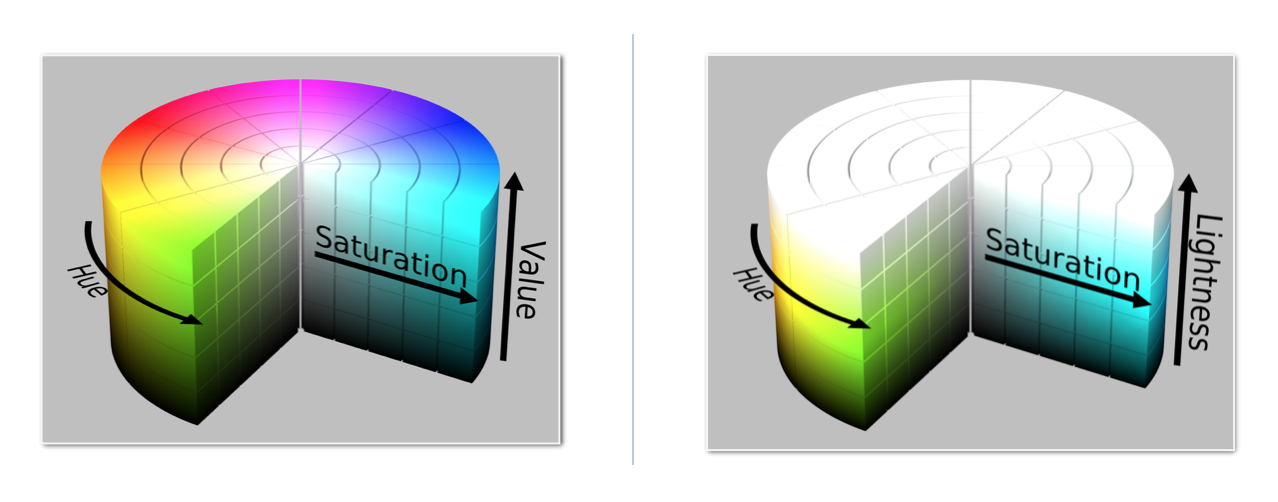
通过 hls = cv2.cvtColor(im, cv2.COLOR_RGB2HLS)可以将RGB修改为HLS颜色空间。
9. HLS intuitions

- A图有最小的L值,即亮度
- A/B/C有相同的色调H。
10. HLS and Color Thresholds HLS颜色空间和颜色阈值
10.1 grayscale
转换成灰度图像后,直接用阈值过滤:
import numpy as np
import cv2
import matplotlib.pyplot as plt
import matplotlib.image as mpimg

image = mpimg.imread('./L10/test6.jpg')
thresh = (180, 255)
gray = cv2.cvtColor(image, cv2.COLOR_RGB2GRAY)
binary = np.zeros_like(gray)
binary[(gray > thresh[0]) & (gray <= thresh[1])] = 1

f, (ax1, ax2) = plt.subplots(1, 2, figsize=(24, 9))
f.tight_layout()
ax1.imshow(gray, cmap='gray')
ax1.set_title('gray Image', fontsize=50)
ax2.imshow(binary, cmap='gray')
ax2.set_title('gray binary Image', fontsize=50)
plt.subplots_adjust(left=0., right=1, top=0.9, bottom=0.)

10.2 individual RGB color channels
下面的代码,都是基于第一部分10.1的代码,将RGB通道颜色值分离,可以看到B下面黄色消失了,说明Brgb(0,0,256)和黄色rgb(256,256,0)叠加后就是黑色。
R = image[:,:,0]
G = image[:,:,1]
B = image[:,:,2]

f, (ax1, ax2, ax3) = plt.subplots(1, 3, figsize=(24, 9))
f.tight_layout()
ax1.imshow(R, cmap='gray')
ax1.set_title('R Image', fontsize=28)

ax2.imshow(G, cmap='gray')
ax2.set_title('G Image', fontsize=28)

ax3.imshow(B, cmap='gray')
ax3.set_title('B Image', fontsize=28)

plt.subplots_adjust(left=0., right=1, top=0.9, bottom=0.)

10.3 R channel与R binary
thresh = (200, 255)
binary = np.zeros_like(R)
binary[(R > thresh[0]) & (R <= thresh[1])] = 1

f, (ax1, ax2) = plt.subplots(1, 2, figsize=(24, 9))
f.tight_layout()
ax1.imshow(R, cmap='gray')
ax1.set_title('R Channel Image', fontsize=50)
ax2.imshow(binary, cmap='gray')
ax2.set_title('R binary Image', fontsize=50)
plt.subplots_adjust(left=0., right=1, top=0.9, bottom=0.)

10.4 HLS
hls = cv2.cvtColor(image, cv2.COLOR_RGB2HLS)
H = hls[:,:,0]
L = hls[:,:,1]
S = hls[:,:,2]

f, (ax1, ax2, ax3) = plt.subplots(1, 3, figsize=(24, 9))
f.tight_layout()
ax1.imshow(H, cmap='gray')
ax1.set_title('H Image', fontsize=28)

ax2.imshow(L, cmap='gray')
ax2.set_title('L Image', fontsize=28)

ax3.imshow(S, cmap='gray')
ax3.set_title('S Image', fontsize=28)

plt.subplots_adjust(left=0., right=1, top=0.9, bottom=0.)

10.5 S channel与S binary
thresh = (90, 255)
binary = np.zeros_like(S)
binary[(S > thresh[0]) & (S <= thresh[1])] = 1

f, (ax1, ax2) = plt.subplots(1, 2, figsize=(24, 9))
f.tight_layout()
ax1.imshow(S, cmap='gray')
ax1.set_title('S Channel Image', fontsize=50)
ax2.imshow(binary, cmap='gray')
ax2.set_title('S binary Image', fontsize=50)
plt.subplots_adjust(left=0., right=1, top=0.9, bottom=0.)

10.6 H channel与H binary
thresh = (15, 100)
binary = np.zeros_like(H)
binary[(H > thresh[0]) & (H <= thresh[1])] = 1

f, (ax1, ax2) = plt.subplots(1, 2, figsize=(24, 9))
f.tight_layout()
ax1.imshow(H, cmap='gray')
ax1.set_title('H Channel Image', fontsize=50)
ax2.imshow(binary, cmap='gray')
ax2.set_title('H binary Image', fontsize=50)
plt.subplots_adjust(left=0., right=1, top=0.9, bottom=0.)

上面可以看出,在S通道下效果是最好的
11. HLS Quiz
import matplotlib.pyplot as plt
import matplotlib.image as mpimg
import numpy as np
import cv2

# Read in an image, you can also try test1.jpg or test4.jpg
image = mpimg.imread('./L10/test6.jpg')

# Define a function that thresholds the S-channel of HLS
# Use exclusive lower bound (>) and inclusive upper (<=)
def hls_select(img, thresh=(0, 255)):
    # 1) Convert to HLS color space
    hls = cv2.cvtColor(image, cv2.COLOR_RGB2HLS)
    S = hls[:,:,2]
    # 2) Apply a threshold to the S channel
    binary_output = np.zeros_like(S)
    binary_output[(S > thresh[0]) & (S <= thresh[1])] = 1

    # 3) Return a binary image of threshold result

    return binary_output

hls_binary = hls_select(image, thresh=(90, 255))

# Plot the result
f, (ax1, ax2) = plt.subplots(1, 2, figsize=(24, 9))
f.tight_layout()
ax1.imshow(image)
ax1.set_title('Original Image', fontsize=50)
ax2.imshow(hls_binary, cmap='gray')
ax2.set_title('Thresholded S', fontsize=50)
plt.subplots_adjust(left=0., right=1, top=0.9, bottom=0.)

12. Color and Gradient
12.1 代码
下面将之前学习到的颜色和梯度结合起来,处理出一个最佳结果.
import numpy as np
import cv2
import matplotlib.pyplot as plt
import matplotlib.image as mpimg


image = mpimg.imread('./L12/bridge_shadow.jpg')

# Edit this function to create your own pipeline.
def pipeline(img, s_thresh=(170, 255), sx_thresh=(20, 100)):
    img = np.copy(img)
    # Convert to HLS color space and separate the V channel
    hls = cv2.cvtColor(img, cv2.COLOR_RGB2HLS)
    s_channel = hls[:,:,2]
    gray = cv2.cvtColor(img, cv2.COLOR_RGB2GRAY)

    # Sobel x
    sobelx = cv2.Sobel(gray, cv2.CV_64F, 1, 0) # Take the derivative in x
    abs_sobelx = np.absolute(sobelx) # Absolute x derivative to accentuate lines away from horizontal
    scaled_sobel = np.uint8(255*abs_sobelx/np.max(abs_sobelx))

    # Threshold x gradient
    sxbinary = np.zeros_like(scaled_sobel)
    sxbinary[(scaled_sobel >= sx_thresh[0]) & (scaled_sobel <= sx_thresh[1])] = 1

    # Threshold color channel
    s_binary = np.zeros_like(s_channel)
    s_binary[(s_channel >= s_thresh[0]) & (s_channel <= s_thresh[1])] = 1
    # Stack each channel
    color_binary = np.dstack(( np.zeros_like(sxbinary), sxbinary, s_binary)) * 255

    # Combine the two binary thresholds
    combined_binary = np.zeros_like(sxbinary)
    combined_binary[(s_binary == 1) | (sxbinary == 1)] = 1

    return combined_binary

result = pipeline(image)

# Plot the result
f, (ax1, ax2) = plt.subplots(1, 2, figsize=(24, 9))
f.tight_layout()

ax1.imshow(image, cmap='gray')
ax1.set_title('Original Image', fontsize=40)

ax2.imshow(result, cmap='gray')
ax2.set_title('Pipeline Result', fontsize=40)
plt.subplots_adjust(left=0., right=1, top=0.9, bottom=0.)
结果如下:

12.2 参考代码
import numpy as np
import cv2
import matplotlib.pyplot as plt
import matplotlib.image as mpimg


img = mpimg.imread('./L12/bridge_shadow.jpg')

# Convert to HLS color space and separate the S channel
# Note: img is the undistorted image
hls = cv2.cvtColor(img, cv2.COLOR_RGB2HLS)
s_channel = hls[:,:,2]

# Grayscale image
# NOTE: we already saw that standard grayscaling lost color information for the lane lines
# Explore gradients in other colors spaces / color channels to see what might work better
gray = cv2.cvtColor(img, cv2.COLOR_RGB2GRAY)

# Sobel x
sobelx = cv2.Sobel(gray, cv2.CV_64F, 1, 0) # Take the derivative in x
abs_sobelx = np.absolute(sobelx) # Absolute x derivative to accentuate lines away from horizontal
scaled_sobel = np.uint8(255*abs_sobelx/np.max(abs_sobelx))

# Threshold x gradient
thresh_min = 20
thresh_max = 100
sxbinary = np.zeros_like(scaled_sobel)
sxbinary[(scaled_sobel >= thresh_min) & (scaled_sobel <= thresh_max)] = 1

# Threshold color channel
s_thresh_min = 170
s_thresh_max = 255
s_binary = np.zeros_like(s_channel)
s_binary[(s_channel >= s_thresh_min) & (s_channel <= s_thresh_max)] = 1

# Stack each channel to view their individual contributions in green and blue respectively
# This returns a stack of the two binary images, whose components you can see as different colors
color_binary = np.dstack(( np.zeros_like(sxbinary), sxbinary, s_binary)) * 255

# Combine the two binary thresholds
combined_binary = np.zeros_like(sxbinary)
combined_binary[(s_binary == 1) | (sxbinary == 1)] = 1

# Plotting thresholded images
f, (ax1, ax2) = plt.subplots(1, 2, figsize=(20,10))
ax1.set_title('Stacked thresholds')
ax1.imshow(color_binary)

ax2.set_title('Combined S channel and gradient thresholds')
ax2.imshow(combined_binary, cmap='gray')

13. 总结
本节从梯度和颜色两方面着手,实现了车道线的提取。

在最后一个练习中,将这两部分的内容糅合起来,得到最好的执行结果。
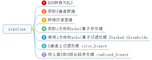
将上面的12.2的最后代码修改为:
f, (ax1, ax2, ax3) = plt.subplots(1, 3, figsize=(24, 9))
f.tight_layout()
ax1.imshow(s_binary, cmap='gray')
ax1.set_title('Stacked thresholds', fontsize=28)

ax2.imshow(color_binary, cmap='gray')
ax2.set_title('color_binary', fontsize=28)

ax3.imshow(combined_binary, cmap='gray')
ax3.set_title('Combined S channel and gradient thresholds', fontsize=28)

plt.subplots_adjust(left=0., right=1, top=0.9, bottom=0.)
描画出上面的⑤⑥⑦,三幅图如下:
