- 1. Reviewing steps
- 2. Processing Each Image
- 3. Finding the Lines:Histogram Peaks(直方图峰值)
- 4. Finding the Lines:Sliding Window(滑动窗口)
- 5. Finding the Lines:Search from Prior
- 6. Another Sliding Window Search 另一种滑动窗口查找
- 7. Measuring Curvature(曲率) I
- 8. Measuring Curvature II
- 9. Bonus Round: Computer Vision [Optional]
- 10. 总结
1. Reviewing steps
Steps we’ve covered so far:
- Camera calibration 校准镜头
- Distortion correction 畸变校正
- Color/gradient threshold 颜色梯度阈值
- Perspective transform 透视变换
After doing these steps, you’ll be given two additional steps for the project:
- Detect lane lines 车线检测
- Determine the lane curvature 计算车线曲率
2. Processing Each Image
首先需要计算镜头的校准矩阵和畸变参数,这个只需要计算一次,然后将其应用到每一帧数据中。然后,使用阈值创建二进制图像,并进行透视变换。
2.1 Thresholding 阈值
可以使用多种不同的颜色和梯度阈值组合,去生成车道线清晰的二进制图像,生成后图象如下:

2.2 Perspective Transform 透视变换
首先要为透视变换找四个点,在以bird view视角查看图像时,这四个点组成一个矩形。如下图示:

2.3 Now for curved lines(曲线)
上面的四个点可以用于对图像进行透视变换(当然前提条件是,其他图像的道路都是在一个平面上,而且摄像头视角没有改变)。
如何评价一个透视变换是否正确,要看透视变换后图像上的车线,是否平行,不管车线是直线还是曲线。
下面将用阈值处理后的二进制图像进行透视变换,如下图中,两条车道线是平行的。

3. Finding the Lines:Histogram Peaks(直方图峰值)
经过上面的处理,得到通过阈值处理后的图像,现在我们要在图像上找出车道线。下面是一种可能的实现方式:
直方图峰值:
经过校准,阈值和透视变换后,我们得到了车道线较为清晰的二进制图像,但是仍然需要识别哪些像素是车道线,哪些是左车线哪些是右车线。
下面是直方图峰值法的代码:
import numpy as np
import matplotlib.image as mpimg
import matplotlib.pyplot as plt

# Load our image
# `mpimg.imread` will load .jpg as 0-255, so normalize back to 0-1
img = mpimg.imread('./L03/warped-example.jpg')/255

def hist(img):
    # TO-DO: Grab only the bottom half of the image
    # Lane lines are likely to be mostly vertical nearest to the car
    bottom_half = img[img.shape[0]//2:,:]

    # Sum across image pixels vertically - make sure to set an `axis`
    # i.e. the highest areas of vertical lines should be larger values
    histogram = np.sum(bottom_half, axis=0)

    return histogram

# Create histogram of image binary activations
histogram = hist(img)

# Visualize the resulting histogram
plt.plot(histogram)
plt.show()
处理后图形为:

看看原始的图像:
import matplotlib.pyplot as plt
import matplotlib.image as mpimg
import numpy as np
%matplotlib inline

img = mpimg.imread('./L03/warped-example.jpg')
bottom_half = img[img.shape[0]//2:,:]


f, (ax1, ax2) = plt.subplots(1, 2, figsize=(24, 10))
ax1.set_title("full image", fontsize=24)
ax1.imshow(img,cmap='gray')
ax2.set_title("bottom_half image", fontsize=24)
ax2.imshow(bottom_half,cmap='gray')

4. Finding the Lines:Sliding Window(滑动窗口)
本节讲述如何通过滑动窗口获得车道线,效果如下:

4.1 实现代码如下:
import numpy as np
import matplotlib.image as mpimg
import matplotlib.pyplot as plt
import cv2

# Load our image
binary_warped = mpimg.imread('./L03/warped-example.jpg')

def find_lane_pixels(binary_warped):
    # Take a histogram of the bottom half of the image
    histogram = np.sum(binary_warped[binary_warped.shape[0]//2:,:], axis=0)
    # Create an output image to draw on and visualize the result
    out_img = np.dstack((binary_warped, binary_warped, binary_warped))
    # Find the peak of the left and right halves of the histogram
    # These will be the starting point for the left and right lines
    midpoint = np.int(histogram.shape[0]//2)
    leftx_base = np.argmax(histogram[:midpoint])
    rightx_base = np.argmax(histogram[midpoint:]) + midpoint

    # HYPERPARAMETERS
    # Choose the number of sliding windows
    nwindows = 9
    # Set the width of the windows +/- margin
    margin = 100
    # Set minimum number of pixels found to recenter window
    minpix = 50

    # Set height of windows - based on nwindows above and image shape
    window_height = np.int(binary_warped.shape[0]//nwindows)
    # Identify the x and y positions of all nonzero pixels in the image
    nonzero = binary_warped.nonzero()
    nonzeroy = np.array(nonzero[0])
    nonzerox = np.array(nonzero[1])
    # Current positions to be updated later for each window in nwindows
    leftx_current = leftx_base
    rightx_current = rightx_base

    # Create empty lists to receive left and right lane pixel indices
    left_lane_inds = []
    right_lane_inds = []

    # Step through the windows one by one
    for window in range(nwindows):
        # Identify window boundaries in x and y (and right and left)
        win_y_low = binary_warped.shape[0] - (window+1)*window_height
        win_y_high = binary_warped.shape[0] - window*window_height
        win_xleft_low = leftx_current - margin
        win_xleft_high = leftx_current + margin
        win_xright_low = rightx_current - margin
        win_xright_high = rightx_current + margin

        # Draw the windows on the visualization image
        cv2.rectangle(out_img,(win_xleft_low,win_y_low),
        (win_xleft_high,win_y_high),(0,255,0), 2)
        cv2.rectangle(out_img,(win_xright_low,win_y_low),
        (win_xright_high,win_y_high),(0,255,0), 2)

        # Identify the nonzero pixels in x and y within the window #
        good_left_inds = ((nonzeroy >= win_y_low) & (nonzeroy < win_y_high) &
        (nonzerox >= win_xleft_low) &  (nonzerox < win_xleft_high)).nonzero()[0]
        good_right_inds = ((nonzeroy >= win_y_low) & (nonzeroy < win_y_high) &
        (nonzerox >= win_xright_low) &  (nonzerox < win_xright_high)).nonzero()[0]

        # Append these indices to the lists
        left_lane_inds.append(good_left_inds)
        right_lane_inds.append(good_right_inds)

        # If you found > minpix pixels, recenter next window on their mean position
        if len(good_left_inds) > minpix:
            leftx_current = np.int(np.mean(nonzerox[good_left_inds]))
        if len(good_right_inds) > minpix:
            rightx_current = np.int(np.mean(nonzerox[good_right_inds]))

    # Concatenate the arrays of indices (previously was a list of lists of pixels)
    try:
        left_lane_inds = np.concatenate(left_lane_inds)
        right_lane_inds = np.concatenate(right_lane_inds)
    except ValueError:
        # Avoids an error if the above is not implemented fully
        pass

    # Extract left and right line pixel positions
    leftx = nonzerox[left_lane_inds]
    lefty = nonzeroy[left_lane_inds]
    rightx = nonzerox[right_lane_inds]
    righty = nonzeroy[right_lane_inds]

    return leftx, lefty, rightx, righty, out_img


def fit_polynomial(binary_warped):
    # Find our lane pixels first
    leftx, lefty, rightx, righty, out_img = find_lane_pixels(binary_warped)

    # Fit a second order polynomial to each using `np.polyfit`
    left_fit = np.polyfit(lefty, leftx, 2)
    right_fit = np.polyfit(righty, rightx, 2)

    # Generate x and y values for plotting
    ploty = np.linspace(0, binary_warped.shape[0]-1, binary_warped.shape[0] )
    try:
        left_fitx = left_fit[0]*ploty**2 + left_fit[1]*ploty + left_fit[2]
        right_fitx = right_fit[0]*ploty**2 + right_fit[1]*ploty + right_fit[2]
    except TypeError:
        # Avoids an error if `left` and `right_fit` are still none or incorrect
        print('The function failed to fit a line!')
        left_fitx = 1*ploty**2 + 1*ploty
        right_fitx = 1*ploty**2 + 1*ploty

    ## Visualization ##
    # Colors in the left and right lane regions
    out_img[lefty, leftx] = [255, 0, 0]
    out_img[righty, rightx] = [0, 0, 255]

    # Plots the left and right polynomials on the lane lines
    plt.plot(left_fitx, ploty, color='yellow')
    plt.plot(right_fitx, ploty, color='yellow')

    return out_img


out_img = fit_polynomial(binary_warped)

plt.imshow(out_img)

4.2 分解直方图(Split the histogram for the two lines)
将直方图分解成两个部分,每个部分对应一条车道线:
import numpy as np
import cv2
import matplotlib.pyplot as plt

binary_warped = mpimg.imread('./L03/warped-example.jpg')/255

# Assuming you have created a warped binary image called "binary_warped"
# Take a histogram of the bottom half of the image
histogram = np.sum(binary_warped[binary_warped.shape[0]//2:,:], axis=0)
# Create an output image to draw on and visualize the result
out_img = np.dstack((binary_warped, binary_warped, binary_warped))*255
# Find the peak of the left and right halves of the histogram
# These will be the starting point for the left and right lines
midpoint = np.int(histogram.shape[0]//2)
leftx_base = np.argmax(histogram[:midpoint])
rightx_base = np.argmax(histogram[midpoint:]) + midpoint

print("left_max_index:",leftx_base," / right_max_index:",rightx_base)
输出 left_max_index: 327 / right_max_index: 971
4.3 设定窗口和窗口的超参数(Set up windows and window hyperparameters)
下一步是设定一些与滑动窗口相关的参数:
# HYPERPARAMETERS
# Choose the number of sliding windows
nwindows = 9
# Set the width of the windows +/- margin
margin = 100
# Set minimum number of pixels found to recenter window
minpix = 50

# Set height of windows - based on nwindows above and image shape
window_height = np.int(binary_warped.shape[0]//nwindows)
# Identify the x and y positions of all nonzero (i.e. activated) pixels in the image
nonzero = binary_warped.nonzero()
nonzeroy = np.array(nonzero[0])
nonzerox = np.array(nonzero[1])
# Current positions to be updated later for each window in nwindows
leftx_current = leftx_base
rightx_current = rightx_base

# Create empty lists to receive left and right lane pixel indices
left_lane_inds = []
right_lane_inds = []
4.4 通过窗口迭代追踪曲率(Iterate through nwindows to track curvature)
- 迭代nwindows
- 知道当前windows的边界
- 使用cv2.rectangle将Windows边界描画到图像上
- 查找窗口中的非0像素点
- 将上述查找到的点添加到
left_lane_inds和right_lane_inds - 如果上面step4中找到的像素数小于参数
minpix,则基于这些像素的位置,重新移动当前Windows。
    # Step through the windows one by one
    for window in range(nwindows):
        # Identify window boundaries in x and y (and right and left)
        win_y_low = binary_warped.shape[0] - (window+1)*window_height
        win_y_high = binary_warped.shape[0] - window*window_height
        win_xleft_low = leftx_current - margin
        win_xleft_high = leftx_current + margin
        win_xright_low = rightx_current - margin
        win_xright_high = rightx_current + margin

        # Draw the windows on the visualization image
        cv2.rectangle(out_img,(win_xleft_low,win_y_low),
        (win_xleft_high,win_y_high),(0,255,0), 2)
        cv2.rectangle(out_img,(win_xright_low,win_y_low),
        (win_xright_high,win_y_high),(0,255,0), 2)

        # Identify the nonzero pixels in x and y within the window #
        good_left_inds = ((nonzeroy >= win_y_low) & (nonzeroy < win_y_high) &
        (nonzerox >= win_xleft_low) &  (nonzerox < win_xleft_high)).nonzero()[0]
        good_right_inds = ((nonzeroy >= win_y_low) & (nonzeroy < win_y_high) &
        (nonzerox >= win_xright_low) &  (nonzerox < win_xright_high)).nonzero()[0]

        # Append these indices to the lists
        left_lane_inds.append(good_left_inds)
        right_lane_inds.append(good_right_inds)

        # If you found > minpix pixels, recenter next window on their mean position
        if len(good_left_inds) > minpix:
            leftx_current = np.int(np.mean(nonzerox[good_left_inds]))
        if len(good_right_inds) > minpix:
            rightx_current = np.int(np.mean(nonzerox[good_right_inds]))
4.5 拟合多项式(Fit a polynomial)
# Concatenate the arrays of indices (previously was a list of lists of pixels)
left_lane_inds = np.concatenate(left_lane_inds)
right_lane_inds = np.concatenate(right_lane_inds)

# Extract left and right line pixel positions
leftx = nonzerox[left_lane_inds]
lefty = nonzeroy[left_lane_inds]
rightx = nonzerox[right_lane_inds]
righty = nonzeroy[right_lane_inds]
# Assuming we have `left_fit` and `right_fit` from `np.polyfit` before
# Generate x and y values for plotting
ploty = np.linspace(0, binary_warped.shape[0]-1, binary_warped.shape[0])
left_fitx = left_fit[0]*ploty**2 + left_fit[1]*ploty + left_fit[2]
right_fitx = right_fit[0]*ploty**2 + right_fit[1]*ploty + right_fit[2]
4.6 Visualization可视化
out_img[lefty, leftx] = [255, 0, 0]
out_img[righty, rightx] = [0, 0, 255]

plt.imshow(out_img)
plt.plot(left_fitx, ploty, color='yellow')
plt.plot(right_fitx, ploty, color='yellow')
plt.xlim(0, 1280)
plt.ylim(720, 0)
Quiz
5. Finding the Lines:Search from Prior
上一节中使用滑动窗口找到了车道线,但是每次都用这种方式去查找车道线太没效率,因为每一帧的图形中,车道线的变化很小。
所以下一帧中,不需要再次进行盲目的查找,可以只查找上一次结果的周边即可,如下图,绿色区域表示本次的查找范围。

5.1 Use the previous polynomial to skip the sliding window
上一部分中,使用left_lane_inds和right_lane_inds保存了落在滑动窗口中像素数据。这一次,使用多项式函数和超参数margin。
5.2 实现代码
import cv2
import numpy as np
import matplotlib.image as mpimg
import matplotlib.pyplot as plt

# Load our image - this should be a new frame since last time!
binary_warped = mpimg.imread('./L03/warped-example.jpg')

# Polynomial fit values from the previous frame
# Make sure to grab the actual values from the previous step in your project!
left_fit = np.array([ 2.13935315e-04, -3.77507980e-01,  4.76902175e+02])
right_fit = np.array([4.17622148e-04, -4.93848953e-01,  1.11806170e+03])

def fit_poly(img_shape, leftx, lefty, rightx, righty):
     ### TO-DO: Fit a second order polynomial to each with np.polyfit() ###
    left_fit = np.polyfit(lefty, leftx, 2)
    right_fit = np.polyfit(righty, rightx, 2)
    # Generate x and y values for plotting
    ploty = np.linspace(0, img_shape[0]-1, img_shape[0])
    ### TO-DO: Calc both polynomials using ploty, left_fit and right_fit ###
    left_fitx = left_fit[0]*ploty**2 + left_fit[1]*ploty + left_fit[2]
    right_fitx = right_fit[0]*ploty**2 + right_fit[1]*ploty + right_fit[2]

    return left_fitx, right_fitx, ploty

def search_around_poly(binary_warped):
    # HYPERPARAMETER
    # Choose the width of the margin around the previous polynomial to search
    # The quiz grader expects 100 here, but feel free to tune on your own!
    margin = 100

    # Grab activated pixels
    nonzero = binary_warped.nonzero()
    nonzeroy = np.array(nonzero[0])
    nonzerox = np.array(nonzero[1])

    ### TO-DO: Set the area of search based on activated x-values ###
    ### within the +/- margin of our polynomial function ###
    ### Hint: consider the window areas for the similarly named variables ###
    ### in the previous quiz, but change the windows to our new search area ###
    left_lane_inds = ((nonzerox > (left_fit[0]*(nonzeroy**2) + left_fit[1]*nonzeroy +
                    left_fit[2] - margin)) & (nonzerox < (left_fit[0]*(nonzeroy**2) +
                    left_fit[1]*nonzeroy + left_fit[2] + margin)))
    right_lane_inds = ((nonzerox > (right_fit[0]*(nonzeroy**2) + right_fit[1]*nonzeroy +
                    right_fit[2] - margin)) & (nonzerox < (right_fit[0]*(nonzeroy**2) +
                    right_fit[1]*nonzeroy + right_fit[2] + margin)))

    # Again, extract left and right line pixel positions
    leftx = nonzerox[left_lane_inds]
    lefty = nonzeroy[left_lane_inds]
    rightx = nonzerox[right_lane_inds]
    righty = nonzeroy[right_lane_inds]

    # Fit new polynomials
    left_fitx, right_fitx, ploty = fit_poly(binary_warped.shape, leftx, lefty, rightx, righty)

    ## Visualization ##
    # Create an image to draw on and an image to show the selection window
    out_img = np.dstack((binary_warped, binary_warped, binary_warped))*255
    window_img = np.zeros_like(out_img)
    # Color in left and right line pixels
    out_img[nonzeroy[left_lane_inds], nonzerox[left_lane_inds]] = [255, 0, 0]
    out_img[nonzeroy[right_lane_inds], nonzerox[right_lane_inds]] = [0, 0, 255]

    # Generate a polygon to illustrate the search window area
    # And recast the x and y points into usable format for cv2.fillPoly()
    left_line_window1 = np.array([np.transpose(np.vstack([left_fitx-margin, ploty]))])
    left_line_window2 = np.array([np.flipud(np.transpose(np.vstack([left_fitx+margin,
                              ploty])))])
    left_line_pts = np.hstack((left_line_window1, left_line_window2))
    right_line_window1 = np.array([np.transpose(np.vstack([right_fitx-margin, ploty]))])
    right_line_window2 = np.array([np.flipud(np.transpose(np.vstack([right_fitx+margin,
                              ploty])))])
    right_line_pts = np.hstack((right_line_window1, right_line_window2))

    # Draw the lane onto the warped blank image
    cv2.fillPoly(window_img, np.int_([left_line_pts]), (0,255, 0))
    cv2.fillPoly(window_img, np.int_([right_line_pts]), (0,255, 0))
    result = cv2.addWeighted(out_img, 1, window_img, 0.3, 0)

    # Plot the polynomial lines onto the image
    plt.plot(left_fitx, ploty, color='yellow')
    plt.plot(right_fitx, ploty, color='yellow')
    ## End visualization steps ##

    return result

# Run image through the pipeline
# Note that in your project, you'll also want to feed in the previous fits
result = search_around_poly(binary_warped)

# View your output
plt.imshow(result)
6. Another Sliding Window Search 另一种滑动窗口查找
另一个滑动窗口查找方式就是使用卷积(convolution),它能将每个窗口中的热点像素最大化放大。一个卷积是两个独立信号内积的和,本示例中是滑动窗口和与其垂直的像素图像切片。(直译过来,懵逼状,不懂)
将滑动窗口从图像的左侧移动到右侧,将所有重叠的元素的和累加,产生卷积信号,重叠最多的像素即卷积信号的峰值,就最可能是车道线。
下面是示例代码:
import numpy as np
import matplotlib.pyplot as plt
import matplotlib.image as mpimg
import glob
import cv2

# Read in a thresholded image
warped = mpimg.imread('./L06/warped_example.jpg')
# window settings
window_width = 50
window_height = 80 # Break image into 9 vertical layers since image height is 720
margin = 100 # How much to slide left and right for searching

def window_mask(width, height, img_ref, center,level):
    output = np.zeros_like(img_ref)
    output[int(img_ref.shape[0]-(level+1)*height):int(img_ref.shape[0]-level*height),max(0,int(center-width/2)):min(int(center+width/2),img_ref.shape[1])] = 1
    return output

def find_window_centroids(image, window_width, window_height, margin):

    window_centroids = [] # Store the (left,right) window centroid positions per level
    window = np.ones(window_width) # Create our window template that we will use for convolutions

    # First find the two starting positions for the left and right lane by using np.sum to get the vertical image slice
    # and then np.convolve the vertical image slice with the window template

    # Sum quarter bottom of image to get slice, could use a different ratio
    l_sum = np.sum(image[int(3*image.shape[0]/4):,:int(image.shape[1]/2)], axis=0)
    l_center = np.argmax(np.convolve(window,l_sum))-window_width/2
    r_sum = np.sum(image[int(3*image.shape[0]/4):,int(image.shape[1]/2):], axis=0)
    r_center = np.argmax(np.convolve(window,r_sum))-window_width/2+int(image.shape[1]/2)

    # Add what we found for the first layer
    window_centroids.append((l_center,r_center))

    # Go through each layer looking for max pixel locations
    for level in range(1,(int)(image.shape[0]/window_height)):
        # convolve the window into the vertical slice of the image
        image_layer = np.sum(image[int(image.shape[0]-(level+1)*window_height):int(image.shape[0]-level*window_height),:], axis=0)
        conv_signal = np.convolve(window, image_layer)
        # Find the best left centroid by using past left center as a reference
        # Use window_width/2 as offset because convolution signal reference is at right side of window, not center of window
        offset = window_width/2
        l_min_index = int(max(l_center+offset-margin,0))
        l_max_index = int(min(l_center+offset+margin,image.shape[1]))
        l_center = np.argmax(conv_signal[l_min_index:l_max_index])+l_min_index-offset
        # Find the best right centroid by using past right center as a reference
        r_min_index = int(max(r_center+offset-margin,0))
        r_max_index = int(min(r_center+offset+margin,image.shape[1]))
        r_center = np.argmax(conv_signal[r_min_index:r_max_index])+r_min_index-offset
        # Add what we found for that layer
        window_centroids.append((l_center,r_center))

    return window_centroids

window_centroids = find_window_centroids(warped, window_width, window_height, margin)

# If we found any window centers
if len(window_centroids) > 0:

    # Points used to draw all the left and right windows
    l_points = np.zeros_like(warped)
    r_points = np.zeros_like(warped)

    # Go through each level and draw the windows
    for level in range(0,len(window_centroids)):
        # Window_mask is a function to draw window areas
        l_mask = window_mask(window_width,window_height,warped,window_centroids[level][0],level)
        r_mask = window_mask(window_width,window_height,warped,window_centroids[level][1],level)
        # Add graphic points from window mask here to total pixels found
        l_points[(l_points == 255) | ((l_mask == 1) ) ] = 255
        r_points[(r_points == 255) | ((r_mask == 1) ) ] = 255

    # Draw the results
    template = np.array(r_points+l_points,np.uint8) # add both left and right window pixels together
    zero_channel = np.zeros_like(template) # create a zero color channel
    template = np.array(cv2.merge((zero_channel,template,zero_channel)),np.uint8) # make window pixels green
    warpage= np.dstack((warped, warped, warped))*255 # making the original road pixels 3 color channels
    output = cv2.addWeighted(warpage, 1, template, 0.5, 0.0) # overlay the orignal road image with window results

# If no window centers found, just display orginal road image
else:
    output = np.array(cv2.merge((warped,warped,warped)),np.uint8)

# Display the final results
plt.imshow(output)
plt.title('window fitting results')
plt.show()

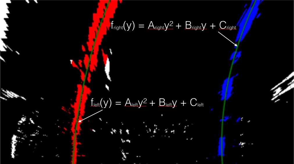
7. Measuring Curvature(曲率) I
通过上面的处理,已经得到了车道线,下图中的红色和蓝色区域,下面需要将这些区域的像素拟合到一个多项式中。
7.1 Radius of Curvature 曲率半径
关于 曲率半径的计算,这里有一篇不错的文章8. Radius of Curvature
import numpy as np

def generate_data():
    '''
    Generates fake data to use for calculating lane curvature.
    In your own project, you'll ignore this function and instead
    feed in the output of your lane detection algorithm to
    the lane curvature calculation.
    '''
    # Set random seed number so results are consistent for grader
    # Comment this out if you'd like to see results on different random data!
    np.random.seed(0)
    # Generate some fake data to represent lane-line pixels
    ploty = np.linspace(0, 719, num=720)# to cover same y-range as image
    quadratic_coeff = 3e-4 # arbitrary quadratic coefficient
    # For each y position generate random x position within +/-50 pix
    # of the line base position in each case (x=200 for left, and x=900 for right)
    leftx = np.array([200 + (y**2)*quadratic_coeff + np.random.randint(-50, high=51)
                                    for y in ploty])
    rightx = np.array([900 + (y**2)*quadratic_coeff + np.random.randint(-50, high=51)
                                    for y in ploty])

    leftx = leftx[::-1]  # Reverse to match top-to-bottom in y
    rightx = rightx[::-1]  # Reverse to match top-to-bottom in y


    # Fit a second order polynomial to pixel positions in each fake lane line
    left_fit = np.polyfit(ploty, leftx, 2)
    right_fit = np.polyfit(ploty, rightx, 2)

    return ploty, left_fit, right_fit

def measure_curvature_pixels():
    '''
    Calculates the curvature of polynomial functions in pixels.
    '''
    # Start by generating our fake example data
    # Make sure to feed in your real data instead in your project!
    ploty, left_fit, right_fit = generate_data()

    # Define y-value where we want radius of curvature
    # We'll choose the maximum y-value, corresponding to the bottom of the image
    y_eval = np.max(ploty)

    # Calculation of R_curve (radius of curvature)
    left_curverad = ((1 + (2*left_fit[0]*y_eval + left_fit[1])**2)**1.5) / np.absolute(2*left_fit[0])
    right_curverad = ((1 + (2*right_fit[0]*y_eval + right_fit[1])**2)**1.5) / np.absolute(2*right_fit[0])

    return left_curverad, right_curverad


# Calculate the radius of curvature in pixels for both lane lines
left_curverad, right_curverad = measure_curvature_pixels()

print(left_curverad, right_curverad)
# Should see values of 1625.06 and 1976.30 here, if using
# the default `generate_data` function with given seed number
输出结果: 1625.06018317 1976.29673077。
8. Measuring Curvature II
基于上面的像素点,计算出了曲率半径,但是这个半径是基于像素空间的,而不是真实空间,所以我们还需要将x和y值转换到真实空间去。
import numpy as np

def generate_data(ym_per_pix, xm_per_pix):
    '''
    Generates fake data to use for calculating lane curvature.
    In your own project, you'll ignore this function and instead
    feed in the output of your lane detection algorithm to
    the lane curvature calculation.
    '''
    # Set random seed number so results are consistent for grader
    # Comment this out if you'd like to see results on different random data!
    np.random.seed(0)
    # Generate some fake data to represent lane-line pixels
    ploty = np.linspace(0, 719, num=720)# to cover same y-range as image
    quadratic_coeff = 3e-4 # arbitrary quadratic coefficient
    # For each y position generate random x position within +/-50 pix
    # of the line base position in each case (x=200 for left, and x=900 for right)
    leftx = np.array([200 + (y**2)*quadratic_coeff + np.random.randint(-50, high=51)
                                    for y in ploty])
    rightx = np.array([900 + (y**2)*quadratic_coeff + np.random.randint(-50, high=51)
                                    for y in ploty])

    leftx = leftx[::-1]  # Reverse to match top-to-bottom in y
    rightx = rightx[::-1]  # Reverse to match top-to-bottom in y

    # Fit a second order polynomial to pixel positions in each fake lane line
    # Fit new polynomials to x,y in world space
    left_fit_cr = np.polyfit(ploty*ym_per_pix, leftx*xm_per_pix, 2)
    right_fit_cr = np.polyfit(ploty*ym_per_pix, rightx*xm_per_pix, 2)

    return ploty, left_fit_cr, right_fit_cr

def measure_curvature_real():
    '''
    Calculates the curvature of polynomial functions in meters.
    '''
    # Define conversions in x and y from pixels space to meters
    ym_per_pix = 30/720 # meters per pixel in y dimension
    xm_per_pix = 3.7/700 # meters per pixel in x dimension

    # Start by generating our fake example data
    # Make sure to feed in your real data instead in your project!
    ploty, left_fit_cr, right_fit_cr = generate_data(ym_per_pix, xm_per_pix)

    # Define y-value where we want radius of curvature
    # We'll choose the maximum y-value, corresponding to the bottom of the image
    y_eval = np.max(ploty)

    # Calculation of R_curve (radius of curvature)
    left_curverad = ((1 + (2*left_fit_cr[0]*y_eval*ym_per_pix + left_fit_cr[1])**2)**1.5) / np.absolute(2*left_fit_cr[0])
    right_curverad = ((1 + (2*right_fit_cr[0]*y_eval*ym_per_pix + right_fit_cr[1])**2)**1.5) / np.absolute(2*right_fit_cr[0])

    return left_curverad, right_curverad


# Calculate the radius of curvature in meters for both lane lines
left_curverad, right_curverad = measure_curvature_real()

print(left_curverad, 'm', right_curverad, 'm')
# Should see values of 533.75 and 648.16 here, if using
# the default `generate_data` function with given seed number
输出结果为: 533.752588921 m 648.157485143 m。
9. Bonus Round: Computer Vision [Optional]
本节是选读部分,介绍了一些车道线检测的论文,以后有需要时过来参考。
10. 总结
本章介绍了后续的两个步骤:
- 车线检测,使用移动窗口的方式计算
- 车线曲率计算,并映射到真实世界空间
本章中涉及的算法较多,没有理解,后续做Project的时候再来回顾理解。