- 1. Tips and Tricks for the Project
- 2. Advanced Lane Finding(概要)
- Step1:Camera Calibration 摄像机标定
- Step2:梯度与颜色空间处理
- step3: 透视变换(bird eye)
- step4:检测车道线
- step5:计算曲率半径和中心偏移
- step6: Set the final pipeline
- step7: Processing the video
- 总结
1. Tips and Tricks for the Project
在本章的学习中,掌握了新的方式去检测和追踪车道线信息,下面是在项目中需要使用的处理方法。
- Camera calibration 摄像头校正
之前的课程和练习中已有涉及了,本项目中使用9×6的棋盘,而不是课程中的8×6。
- 计算出来的斜率是否正确
计算出来的半径应该接近1km。
- 偏移 offset
假设摄像头假设在车的中心部分,那么图像上检测出的两条车道线的中点,就是车道线的中心。从图像中心到车道线中心的偏移,就是车到车道线中心线的距离。
如下图,紫色圆点是车道线中心,黄色圆点是自车位置:

- 追踪
在测试图像上完成pipeline的创建后,我们要将其应用在video流上。
- Sanity(头脑清楚的) Check
往下一步之前,需要对检测结果进行check,检查如下结果:
- 是否有类似的斜率
- 是否它们是否被近似的正确的水平距离所分开 (懵逼状,啥意思…)
- 是否近似的平行
- Look-Ahead(有预见性的) Filter
一旦在video的一帧图像中找到了车道线,而且相当自信找到的车道线是正确的,那么在下一帧图像中可以不需要盲找。
比如,如果匹配了一个多项式,那么对于每个y的位置,都有一个x位置可以表示其车道线中心。
-
Reset
-
平滑处理
-
描画
# Create an image to draw the lines on
warp_zero = np.zeros_like(warped).astype(np.uint8)
color_warp = np.dstack((warp_zero, warp_zero, warp_zero))

# Recast the x and y points into usable format for cv2.fillPoly()
pts_left = np.array([np.transpose(np.vstack([left_fitx, ploty]))])
pts_right = np.array([np.flipud(np.transpose(np.vstack([right_fitx, ploty])))])
pts = np.hstack((pts_left, pts_right))

# Draw the lane onto the warped blank image
cv2.fillPoly(color_warp, np.int_([pts]), (0,255, 0))

# Warp the blank back to original image space using inverse perspective matrix (Minv)
newwarp = cv2.warpPerspective(color_warp, Minv, (image.shape[1], image.shape[0]))
# Combine the result with the original image
result = cv2.addWeighted(undist, 1, newwarp, 0.3, 0)
plt.imshow(result)
2. Advanced Lane Finding(概要)
这个项目中要完成的工作如下:
- 摄像机标定,计算出标定矩阵和校正参数(使用围棋格数据),参考
- 将上面计算的参数应用到道路数据中,对数据实施纠正处理,参考
- 使用color transforms, gradients 等生成 thresholded binary image,参考
- 使用birds-eye对上面的binary image进行视角变换,参考
- 检测lane pixel,参考
- 计算lane的曲率半径以及自车的lane中心偏移,参考
- 将检测到的lane,描画到原始图像中
- 将lane曲率半径以及lane中心偏移距离,显示在原始图像中
- 处理video
步骤以及结果,参考下面的图:
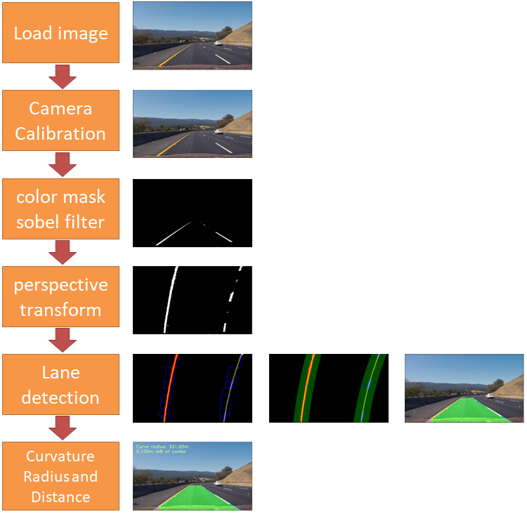
Step1:Camera Calibration 摄像机标定
由于相机的凸出,所以会产生畸变,如下图所示,走道的栏杆是笔直延伸的,但是看上去确实弯曲的,这就是图像畸变,畸变导致图像失真。

使用有畸变的图像做车道线检测,检测结果的精度将会受到影响,因此进行图像处理第一步就是去除畸变。
为了解决摄像机图像的畸变问题,摄像机标定技术产生了,摄像机标定是通过对已知的形状进行拍摄,通过计算该形状在真实世界中的位置与在图像中的位置的偏差量,即畸变参数,从而用这个偏差量去修正其他畸变图像。
通常的标定方法都是基于棋盘格,因为它具备规则的高对比度,能非常方便的自动化检测各个棋盘的交点,十分适合标定摄像机的标定。
代码如下:
import numpy as np
import cv2
import glob
import matplotlib.pyplot as plt
import matplotlib.image as mpimg
import os
%matplotlib inline

nx = 9
ny = 6

# prepare object points, like (0,0,0), (1,0,0), (2,0,0) ....,(6,5,0)
objp = np.zeros((ny*nx,3), np.float32)
objp[:,:2] = np.mgrid[0:nx,0:ny].T.reshape(-1,2)

# Arrays to store object points and image points from all the images.
objpoints = [] # 3d points in real world space
imgpoints = [] # 2d points in image plane.

# Make a list of calibration images
images = glob.glob('./camera_cal/calibration2.jpg')

def cal_undistort(img, objpoints, imgpoints):
    # Use cv2.calibrateCamera() and cv2.undistort()
    gray = cv2.cvtColor(img,cv2.COLOR_BGR2GRAY)
    ret, mtx, dist, rvecs, tvecs = cv2.calibrateCamera(objpoints, imgpoints, gray.shape[::-1], None, None)

    undist = cv2.undistort(img, mtx, dist, None, mtx)
    return undist


# Step through the list and search for chessboard corners
for fname in images:
    img = cv2.imread(fname)
    gray = cv2.cvtColor(img,cv2.COLOR_BGR2GRAY)

    # Find the chessboard corners
    ret, corners = cv2.findChessboardCorners(gray, (nx,ny),None)

    # If found, add object points, image points
    if ret == True:
        objpoints.append(objp)
        imgpoints.append(corners)

        img_corners = np.copy(img)
        img_corners = cv2.drawChessboardCorners(img_corners, (nx,ny), corners, ret)

        undist = cal_undistort(img, objpoints, imgpoints)

        f, (ax1, ax2, ax3) = plt.subplots(1, 3, figsize=(16,4))

        ax1.imshow(cv2.cvtColor(img, cv2.COLOR_BGR2RGB))
        ax1.set_title('Original Image', fontsize=18)

        ax2.imshow(cv2.cvtColor(img_corners, cv2.COLOR_BGR2RGB))
        ax2.set_title('With Corners', fontsize=20)

        ax3.imshow(cv2.cvtColor(undist, cv2.COLOR_BGR2RGB))
        ax3.set_title('Undistorted image', fontsize=20)

        filename = os.path.basename(fname)
        filename = os.path.splitext(filename)[0]
        plt.savefig('./output_images/' + "step1_undistorted_" + filename + '.jpg')

- findChessboardCorners(),自动地检测棋盘格内4个棋盘格的交点(2白2黑的交接点),需要输入摄像机拍摄的完整棋盘格图像和交点在横纵向上的数量.
- 如果找到的话,就将对应点的图像位置,存储到 imgpoints中,objpoints中存储的是规则的矩阵np.zeros((ny*nx,3), np.float32)。
- drawChessboardCorners(img_corners, (nx,ny), corners, ret),描画检测到的交点。
- 使用得到的对比矩阵和函数cal_undistort(),得到纠正后的图像。
使用上面的棋盘得到对应的矩阵后,将其应用到实际的道路数据中,代码如下:
images = glob.glob('./test_images/test3.jpg')
for fname in images:
    img = cv2.imread(fname)
    undist = cal_undistort(img, objpoints, imgpoints)

    f, (ax1, ax2) = plt.subplots(1, 2, figsize=(16,4))

    ax1.imshow(cv2.cvtColor(img, cv2.COLOR_BGR2RGB))
    ax1.set_title('Original Image', fontsize=18)

    ax2.imshow(cv2.cvtColor(undist, cv2.COLOR_BGR2RGB))
    ax2.set_title('Undistorted image', fontsize=20)

    filename = os.path.basename(fname)
    filename = os.path.splitext(filename)[0]
    plt.savefig('./output_images/' + "step1_undistorted_" + filename + '.jpg')

Step2:梯度与颜色空间处理
在道路图像上,真正感兴趣的是车道线,不是周边的树和车,所以我们要用梯度和颜色过滤掉不需要的信息,过滤的时候就需要考虑车道线的特征:
- 颜色: 白色或黄色
- 角度:有一定的角度
代码如下:
def get_thresholded_image(img):
    # convert to gray scale
    gray = cv2.cvtColor(img, cv2.COLOR_RGB2GRAY)

    height, width = gray.shape

    # apply gradient threshold on the horizontal gradient
    sx_binary = abs_sobel_thresh(gray, 'x', 10, 200)

    # apply gradient direction threshold so that only edges closer to vertical are detected.
    dir_binary = dir_threshold(gray, thresh=(np.pi/6, np.pi/2))

    # combine the gradient and direction thresholds.
    combined_condition = ((sx_binary == 1) & (dir_binary == 1))

    # R & G thresholds so that yellow lanes are detected well.
    color_threshold = 150
    R = img[:,:,0]
    G = img[:,:,1]
    color_combined = np.zeros_like(R)
    r_g_condition = (R > color_threshold) & (G > color_threshold)


    # color channel thresholds
    hls = cv2.cvtColor(img, cv2.COLOR_RGB2HLS)
    S = hls[:,:,2]
    L = hls[:,:,1]

    # S channel performs well for detecting bright yellow and white lanes
    s_thresh = (100, 255)
    s_condition = (S > s_thresh[0]) & (S <= s_thresh[1])

    # We put a threshold on the L channel to avoid pixels which have shadows and as a result darker.
    l_thresh = (120, 255)
    l_condition = (L > l_thresh[0]) & (L <= l_thresh[1])

    # combine all the thresholds
    # A pixel should either be a yellowish or whiteish
    # And it should also have a gradient, as per our thresholds
    color_combined[(r_g_condition & l_condition) & (s_condition | combined_condition)] = 1

    # apply the region of interest mask
    mask = np.zeros_like(color_combined)
    region_of_interest_vertices = np.array([[0,height-1], [width/2, int(0.5*height)], [width-1, height-1]], dtype=np.int32)
    cv2.fillPoly(mask, [region_of_interest_vertices], 1)
    thresholded = cv2.bitwise_and(color_combined, mask)

    return thresholded

def abs_sobel_thresh(gray, orient='x', thresh_min=0, thresh_max=255):
    if orient == 'x':
        sobel = cv2.Sobel(gray, cv2.CV_64F, 1, 0)
    else:
        sobel = cv2.Sobel(gray, cv2.CV_64F, 0, 1)
    abs_sobel = np.absolute(sobel)
    max_value = np.max(abs_sobel)
    binary_output = np.uint8(255*abs_sobel/max_value)
    threshold_mask = np.zeros_like(binary_output)
    threshold_mask[(binary_output >= thresh_min) & (binary_output <= thresh_max)] = 1
    return threshold_mask

def dir_threshold(gray, sobel_kernel=3, thresh=(0, np.pi/2)):
    # Take the gradient in x and y separately
    sobel_x = cv2.Sobel(gray, cv2.CV_64F, 1, 0, ksize=sobel_kernel)
    sobel_y = cv2.Sobel(gray, cv2.CV_64F, 0, 1, ksize=sobel_kernel)
    # 3) Take the absolute value of the x and y gradients
    abs_sobel_x = np.absolute(sobel_x)
    abs_sobel_y = np.absolute(sobel_y)
    # 4) Use np.arctan2(abs_sobely, abs_sobelx) to calculate the direction of the gradient
    direction = np.arctan2(abs_sobel_y,abs_sobel_x)
    direction = np.absolute(direction)
    # 5) Create a binary mask where direction thresholds are met
    mask = np.zeros_like(direction)
    mask[(direction >= thresh[0]) & (direction <= thresh[1])] = 1
    # 6) Return this mask as your binary_output image
    return mask


#cv2.imwrite('thresholded.jpg',thresholded)

# Plot the 2 images side by side
images = glob.glob('./test_images/test3.jpg')
for fname in images:
    image = mpimg.imread(fname)
    undist = cal_undistort(image, objpoints, imgpoints)
    thresholded = get_thresholded_image(undist)

    f, (ax1, ax2) = plt.subplots(1, 2, figsize=(24, 9))
    f.tight_layout()
    ax1.imshow(image)
    ax1.set_title('Original Image', fontsize=50)
    ax2.imshow(thresholded, cmap='gray')
    ax2.set_title('Thresholded Image', fontsize=50)
    plt.subplots_adjust(left=0., right=1, top=0.9, bottom=0.)

    filename = os.path.basename(fname)
    filename = os.path.splitext(filename)[0]
    plt.savefig('./output_images/' + "step2_thresholded_" + filename + '.jpg')

1. 根据角度处理
def dir_threshold(gray, sobel_kernel=3, thresh=(0, np.pi/2)):
    # Take the gradient in x and y separately
    sobel_x = cv2.Sobel(gray, cv2.CV_64F, 1, 0, ksize=sobel_kernel)
    sobel_y = cv2.Sobel(gray, cv2.CV_64F, 0, 1, ksize=sobel_kernel)
    # 3) Take the absolute value of the x and y gradients
    abs_sobel_x = np.absolute(sobel_x)
    abs_sobel_y = np.absolute(sobel_y)
    # 4) Use np.arctan2(abs_sobely, abs_sobelx) to calculate the direction of the gradient
    direction = np.arctan2(abs_sobel_y,abs_sobel_x)
    direction = np.absolute(direction)
    # 5) Create a binary mask where direction thresholds are met
    mask = np.zeros_like(direction)
    mask[(direction >= thresh[0]) & (direction <= thresh[1])] = 1
    # 6) Return this mask as your binary_output image
    return mask

... ...

dir_binary = dir_threshold(gray, thresh=(np.pi/6, np.pi/2))
2. sobel算子处理
def abs_sobel_thresh(gray, orient='x', thresh_min=0, thresh_max=255):
    if orient == 'x':
        sobel = cv2.Sobel(gray, cv2.CV_64F, 1, 0)
    else:
        sobel = cv2.Sobel(gray, cv2.CV_64F, 0, 1)
    abs_sobel = np.absolute(sobel)
    max_value = np.max(abs_sobel)
    binary_output = np.uint8(255*abs_sobel/max_value)
    threshold_mask = np.zeros_like(binary_output)
    threshold_mask[(binary_output >= thresh_min) & (binary_output <= thresh_max)] = 1
    return threshold_mask

... ...
sx_binary = abs_sobel_thresh(gray, 'x', 10, 200)
3. 颜色处理
    # R & G thresholds so that yellow lanes are detected well.
    color_threshold = 150
    R = img[:,:,0]
    G = img[:,:,1]
    color_combined = np.zeros_like(R)
    r_g_condition = (R > color_threshold) & (G > color_threshold)


    # color channel thresholds
    hls = cv2.cvtColor(img, cv2.COLOR_RGB2HLS)
    S = hls[:,:,2]
    L = hls[:,:,1]

    # S channel performs well for detecting bright yellow and white lanes
    s_thresh = (100, 255)
    s_condition = (S > s_thresh[0]) & (S <= s_thresh[1])

    # We put a threshold on the L channel to avoid pixels which have shadows and as a result darker.
    l_thresh = (120, 255)
    l_condition = (L > l_thresh[0]) & (L <= l_thresh[1])
step3: 透视变换(bird eye)
“透视”是图像成像时,物体距离摄像机越远,看起来越小的一种现象。在真实世界中,左右互相平行的车道线,会在图像的最远处交汇成一个点。这个现象就是“透视成像”的原理造成的。
通过使用透视变换技术,可以将不规则的八边形投影成规则的正八边形。应用透视变换后的结果对比如下:

透视变换的原理: 首先新建一副跟左图一样的右图,随后在图中选择标志牌位于两侧的四个点,记录这四个点的坐标,原图为srcpoint。在新图中选择一个长方形区域,这四个端点一一对应原图的srcpoint,这四个新的点为dstpoint,得到这新旧的点后,用 cv2.getPerspectiveTransform(src_points, dst_points),就能得到投影矩阵和投影变换后的图像了。
def birds_eye(img):
    img_size = (img.shape[1],img.shape[0])

    src = np.float32(
        [[585,460],
         [203,720],
         [695,460],
         [1127,720]]
    )
    dst = np.float32(
        [[320,0],
         [320,720],
         [960,0],
         [960,720]]
    )

    M = cv2.getPerspectiveTransform(src,dst)
    Minv = cv2.getPerspectiveTransform(dst, src)
    warped = cv2.warpPerspective(img,M,img_size,flags=cv2.INTER_LINEAR)

    return warped,M,Minv

images = glob.glob('./test_images/test3.jpg')
for fname in images:
    image = mpimg.imread(fname)
    combined_binary = get_thresholded_image(image)
    warped,M,Minv = birds_eye(combined_binary)

    f, (ax1, ax2) = plt.subplots(1, 2, figsize=(16,4))

    ax1.imshow(combined_binary, cmap='gray')
    ax1.set_title('bianary', fontsize=18)

    ax2.imshow(warped, cmap='gray')
    ax2.set_title('birds eye image', fontsize=20)

    filename = os.path.basename(fname)
    filename = os.path.splitext(filename)[0]
    plt.savefig('./output_images/' + "step3_birds-eye_" + filename + '.jpg')

step4:检测车道线
1. 直方图
要处理的图像的分辨率是1280*70,如果将每一列白色的点数量进行统计,即可以得到1280个值,将这1280个值绘制在一个坐标系中,横坐标为1-1280,纵坐标为白色点的数量,这个图就是直方图,代码及效果如下:
def hist(img):
    # Lane lines are likely to be mostly vertical nearest to the car
    bottom_half = img[img.shape[0]//2:,:]

    # Sum across image pixels vertically - make sure to set an `axis`
    # i.e. the highest areas of vertical lines should be larger values
    histogram = np.sum(bottom_half, axis=0)

    return histogram

# Visualize the resulting histogram
images = glob.glob('./test_images/test3.jpg')
for fname in images:
    image = mpimg.imread(fname)
    combined_binary = get_thresholded_image(image)
    warped,M,Minv = birds_eye(combined_binary)

    histogram = hist(warped)
    plt.plot(histogram)
    plt.show()

找到直方图左半边最大值所对应的列数,即为左车道线所在的大致位置;找到直方图右半边最大值所对应的列数,即为右车道线所在的大致位置。
2. 滑动窗口法
leftx_base和rightx_base即为左右车道线所在列的大致位置。 确定了左右车道线的大致位置后,使用一种叫做“滑动窗口”的技术,在图中对左右车道线的点进行搜索。
def fit_lines(warped,show=False):
    histogram = hist(warped)

    # Peak in the first half indicates the likely position of the left lane
    half_width = np.int(histogram.shape[0]//2)
    leftx_base = np.argmax(histogram[:half_width])

    # Peak in the second half indicates the likely position of the right lane
    rightx_base = np.argmax(histogram[half_width:]) + half_width

    out_img = np.dstack((warped, warped, warped))*255

    non_zeros = warped.nonzero()
    non_zeros_y = non_zeros[0]
    non_zeros_x = non_zeros[1]

    num_windows = 10
    num_rows = warped.shape[0]
    window_height = np.int(num_rows/num_windows)
    window_half_width = 50

    min_pixels = 100

    left_coordinates = []
    right_coordinates = []

    for window in range(num_windows):
        y_max = num_rows - window*window_height
        y_min = num_rows - (window+1)* window_height

        left_x_min = leftx_base - window_half_width
        left_x_max = leftx_base + window_half_width

        cv2.rectangle(out_img, (left_x_min, y_min), (left_x_max, y_max), [0,0,255],2)

        good_left_window_coordinates = ((non_zeros_x >= left_x_min) & (non_zeros_x <= left_x_max) & (non_zeros_y >= y_min) & (non_zeros_y <= y_max)).nonzero()[0]
        left_coordinates.append(good_left_window_coordinates)

        if len(good_left_window_coordinates) > min_pixels:
            leftx_base = np.int(np.mean(non_zeros_x[good_left_window_coordinates]))

        right_x_min = rightx_base - window_half_width
        right_x_max = rightx_base + window_half_width

        cv2.rectangle(out_img, (right_x_min, y_min), (right_x_max, y_max), [0,0,255],2)

        good_right_window_coordinates = ((non_zeros_x >= right_x_min) & (non_zeros_x <= right_x_max) & (non_zeros_y >= y_min) & (non_zeros_y <= y_max)).nonzero()[0]
        right_coordinates.append(good_right_window_coordinates)

        if len(good_right_window_coordinates) > min_pixels:
            rightx_base = np.int(np.mean(non_zeros_x[good_right_window_coordinates]))

    left_coordinates = np.concatenate(left_coordinates)
    right_coordinates = np.concatenate(right_coordinates)

    out_img[non_zeros_y[left_coordinates], non_zeros_x[left_coordinates]] = [255,0,0]
    out_img[non_zeros_y[right_coordinates], non_zeros_x[right_coordinates]] = [0,0,255]

    left_x = non_zeros_x[left_coordinates]
    left_y = non_zeros_y[left_coordinates]

    polyfit_left = np.polyfit(left_y, left_x, 2)

    right_x = non_zeros_x[right_coordinates]
    right_y = non_zeros_y[right_coordinates]

    polyfit_right = np.polyfit(right_y, right_x, 2)

    y_points = np.linspace(0, num_rows-1, num_rows)

    left_x_predictions = polyfit_left[0]*y_points**2 + polyfit_left[1]*y_points + polyfit_left[2]

    right_x_predictions = polyfit_right[0]*y_points**2 + polyfit_right[1]*y_points + polyfit_right[2]

    if show == True:
        plt.imshow(out_img)
        plt.plot(left_x_predictions, y_points, color='yellow')
        plt.plot(right_x_predictions, y_points, color='yellow')
        plt.xlim(0, warped.shape[1])
        plt.ylim(warped.shape[0],0)

    return polyfit_left,polyfit_right

- 首先根据前面介绍的直方图方法,找到左右车道车线的大致位置,将这两个大致位置作为起始点,定义一个矩形区域,称为窗口。分别以这两个起始点作为窗口的下边线中点,存储所有在方块中的白色点的横坐标。

- 随后对存储的横坐标取均值,将该均值所在的列以及第一个窗口的上边缘所在的位置,作为下一个窗口的下边线中点,继续搜索。

- 依次往复,至到把所有的行都搜索完毕。

- 所有落在窗口(图中棕色区域)中的白点,即为左右车道线的待选点,如下图蓝色和红色所示。随后将蓝色点和红色点做三次曲线拟合,即可得到车道线的曲线方程。

3. 跟踪车道线
视频数据是连续的图片,基于连续两帧图像中的车道线不会突变,我们可以使用上一帧检测得到的车线结果,作为下一帧图像处理的输入,搜索上一帧车道线的检测结果附近的点,这样不仅可以减少计算量,而且得到的车道线结果也更稳定。

上图中细黄线为上一帧检测到的车道线结果,绿色阴影为细黄线横向扩展的一个区域,通过搜索该区域内的白点坐标,即可快速确定当前帧中左右车道线的待选点。
代码如下:
def fit_poly(img_shape, leftx, lefty, rightx, righty):
     ### TO-DO: Fit a second order polynomial to each with np.polyfit() ###
    left_fit = np.polyfit(lefty, leftx, 2)
    right_fit = np.polyfit(righty, rightx, 2)
    # Generate x and y values for plotting
    ploty = np.linspace(0, img_shape[0]-1, img_shape[0])
    ### TO-DO: Calc both polynomials using ploty, left_fit and right_fit ###
    left_fitx = left_fit[0]*ploty**2 + left_fit[1]*ploty + left_fit[2]
    right_fitx = right_fit[0]*ploty**2 + right_fit[1]*ploty + right_fit[2]

    return left_fitx, right_fitx, ploty

def search_around_poly(binary_warped,left_fit,right_fit,show=False):
    # HYPERPARAMETER
    # Choose the width of the margin around the previous polynomial to search
    # The quiz grader expects 100 here, but feel free to tune on your own!
    margin = 80

    # Grab activated pixels
    nonzero = binary_warped.nonzero()
    nonzeroy = np.array(nonzero[0])
    nonzerox = np.array(nonzero[1])

    ### TO-DO: Set the area of search based on activated x-values ###
    ### within the +/- margin of our polynomial function ###
    ### Hint: consider the window areas for the similarly named variables ###
    ### in the previous quiz, but change the windows to our new search area ###
    left_lane_inds = ((nonzerox > (left_fit[0]*(nonzeroy**2) + left_fit[1]*nonzeroy +
                    left_fit[2] - margin)) & (nonzerox < (left_fit[0]*(nonzeroy**2) +
                    left_fit[1]*nonzeroy + left_fit[2] + margin)))
    right_lane_inds = ((nonzerox > (right_fit[0]*(nonzeroy**2) + right_fit[1]*nonzeroy +
                    right_fit[2] - margin)) & (nonzerox < (right_fit[0]*(nonzeroy**2) +
                    right_fit[1]*nonzeroy + right_fit[2] + margin)))

    # Again, extract left and right line pixel positions
    leftx = nonzerox[left_lane_inds]
    lefty = nonzeroy[left_lane_inds]
    rightx = nonzerox[right_lane_inds]
    righty = nonzeroy[right_lane_inds]

    # Fit new polynomials
    left_fitx, right_fitx, ploty = fit_poly(binary_warped.shape, leftx, lefty, rightx, righty)

    ## Visualization ##
    # Create an image to draw on and an image to show the selection window
    out_img = np.dstack((binary_warped, binary_warped, binary_warped))*255
    window_img = np.zeros_like(out_img)
    # Color in left and right line pixels

    out_img[nonzeroy[left_lane_inds], nonzerox[left_lane_inds]] = [255, 0, 0]
    out_img[nonzeroy[right_lane_inds], nonzerox[right_lane_inds]] = [0, 0, 255]

    # Generate a polygon to illustrate the search window area
    # And recast the x and y points into usable format for cv2.fillPoly()
    left_line_window1 = np.array([np.transpose(np.vstack([left_fitx-margin, ploty]))])
    left_line_window2 = np.array([np.flipud(np.transpose(np.vstack([left_fitx+margin,
                              ploty])))])
    left_line_pts = np.hstack((left_line_window1, left_line_window2))
    right_line_window1 = np.array([np.transpose(np.vstack([right_fitx-margin, ploty]))])
    right_line_window2 = np.array([np.flipud(np.transpose(np.vstack([right_fitx+margin,
                              ploty])))])
    right_line_pts = np.hstack((right_line_window1, right_line_window2))

    # Draw the lane onto the warped blank image
    cv2.fillPoly(window_img, np.int_([left_line_pts]), (0,255, 0))
    cv2.fillPoly(window_img, np.int_([right_line_pts]), (0,255, 0))
    result = cv2.addWeighted(out_img, 1, window_img, 0.3, 0)

    if show == True:
        # Plot the polynomial lines onto the image
        plt.plot(left_fitx, ploty, color='yellow')
        plt.plot(right_fitx, ploty, color='yellow')
        ## End visualization steps ##

    return result,left_fitx, right_fitx, ploty,left_lane_inds,right_lane_inds

fname = './test_images/test3.jpg'
image = mpimg.imread(fname)
combined_binary = get_thresholded_image(image)
warped,M,Minv = birds_eye(combined_binary)

left_fit,right_fit = fit_lines(warped)

result,left_fitx, right_fitx, ploty,left_lane_inds,right_lane_inds = search_around_poly(warped,left_fit,right_fit,True)
plt.imshow(result)
4. 逆投影到原图
我们在计算透视变换矩阵时计算了两个矩阵M和Minv,使用M能够实现透视变换,使用Minv能够实现逆向透视变换。
M = cv2.getPerspectiveTransform(src,dst)
Minv = cv2.getPerspectiveTransform(dst, src)
我们将两条车道线所围成的区域涂成绿色,并将结果绘制到鸟瞰图上,使用逆透视变换矩阵反投到原图上,即可以实现原图的可视化效果,代码如下:
def draw_lane(original_img, binary_img, l_fit, r_fit, Minv):
    new_img = np.copy(original_img)
    if l_fit is None or r_fit is None:
        return original_img
    # Create an image to draw the lines on
    warp_zero = np.zeros_like(binary_img).astype(np.uint8)
    color_warp = np.dstack((warp_zero, warp_zero, warp_zero))

    h,w = binary_img.shape
    ploty = np.linspace(0, h-1, num=h)# to cover same y-range as image
    left_fitx = l_fit[0]*ploty**2 + l_fit[1]*ploty + l_fit[2]
    right_fitx = r_fit[0]*ploty**2 + r_fit[1]*ploty + r_fit[2]

    # Recast the x and y points into usable format for cv2.fillPoly()
    pts_left = np.array([np.transpose(np.vstack([left_fitx, ploty]))])
    pts_right = np.array([np.flipud(np.transpose(np.vstack([right_fitx, ploty])))])
    pts = np.hstack((pts_left, pts_right))

    # Draw the lane onto the warped blank image
    cv2.fillPoly(color_warp, np.int_([pts]), (0,255, 0))
    cv2.polylines(color_warp, np.int32([pts_left]), isClosed=False, color=(255,0,255), thickness=15)
    cv2.polylines(color_warp, np.int32([pts_right]), isClosed=False, color=(0,255,255), thickness=15)

    # Warp the blank back to original image space using inverse perspective matrix (Minv)
    newwarp = cv2.warpPerspective(color_warp, Minv, (w, h))
    # Combine the result with the original image
    result = cv2.addWeighted(new_img, 1, newwarp, 0.5, 0)
    return result

exampleImg_out1 = draw_lane(image, warped, left_fit, right_fit, Minv)

f, (ax1, ax2) = plt.subplots(1, 2, figsize=(16,4))

ax1.imshow(image, cmap='gray')
ax1.set_title('image', fontsize=18)

ax2.imshow(exampleImg_out1, cmap='gray')
ax2.set_title('lane detected image', fontsize=20)

filename = os.path.basename(fname)
filename = os.path.splitext(filename)[0]
plt.savefig('./output_images/' + "step4_" + filename + '.jpg')

step5:计算曲率半径和中心偏移
关于曲率半径相关公式和推导,可以参考这里
# Method to determine radius of curvature and distance from lane center
# based on binary image, polynomial fit, and L and R lane pixel indices
def calc_curv_rad_and_center_dist(bin_img, l_fit, r_fit, l_lane_inds, r_lane_inds):
    # Define conversions in x and y from pixels space to meters
    ym_per_pix = 3.048/100 # meters per pixel in y dimension, lane line is 10 ft = 3.048 meters
    xm_per_pix = 3.7/378 # meters per pixel in x dimension, lane width is 12 ft = 3.7 meters
    left_curverad, right_curverad, center_dist = (0, 0, 0)
    # Define y-value where we want radius of curvature
    # I'll choose the maximum y-value, corresponding to the bottom of the image
    h = bin_img.shape[0]
    ploty = np.linspace(0, h-1, h)
    y_eval = np.max(ploty)

    # Identify the x and y positions of all nonzero pixels in the image
    nonzero = bin_img.nonzero()
    nonzeroy = np.array(nonzero[0])
    nonzerox = np.array(nonzero[1])
    # Again, extract left and right line pixel positions
    leftx = nonzerox[l_lane_inds]
    lefty = nonzeroy[l_lane_inds]
    rightx = nonzerox[r_lane_inds]
    righty = nonzeroy[r_lane_inds]

    if len(leftx) != 0 and len(rightx) != 0:
        # Fit new polynomials to x,y in world space
        left_fit_cr = np.polyfit(lefty*ym_per_pix, leftx*xm_per_pix, 2)
        right_fit_cr = np.polyfit(righty*ym_per_pix, rightx*xm_per_pix, 2)
        # Calculate the new radii of curvature
        left_curverad = ((1 + (2*left_fit_cr[0]*y_eval*ym_per_pix + left_fit_cr[1])**2)**1.5) / np.absolute(2*left_fit_cr[0])
        right_curverad = ((1 + (2*right_fit_cr[0]*y_eval*ym_per_pix + right_fit_cr[1])**2)**1.5) / np.absolute(2*right_fit_cr[0])
        # Now our radius of curvature is in meters

    # Distance from center is image x midpoint - mean of l_fit and r_fit intercepts
    if r_fit is not None and l_fit is not None:
        car_position = bin_img.shape[1]/2
        l_fit_x_int = l_fit[0]*h**2 + l_fit[1]*h + l_fit[2]
        r_fit_x_int = r_fit[0]*h**2 + r_fit[1]*h + r_fit[2]
        lane_center_position = (r_fit_x_int + l_fit_x_int) /2
        center_dist = (car_position - lane_center_position) * xm_per_pix
    return left_curverad, right_curverad, center_dist

combined_binary = get_thresholded_image(image)
warped,M,Minv = birds_eye(combined_binary)

left_fit,right_fit = fit_lines(warped)

rad_l, rad_r, d_center = calc_curv_rad_and_center_dist(warped, left_fit, right_fit, left_lane_inds, right_lane_inds)

print('Radius of curvature for example:', rad_l, 'm,', rad_r, 'm')
print('Distance from lane center for example:', d_center, 'm')
将结果绘制到原图上去:
def draw_data(original_img, curv_rad, center_dist):
    new_img = np.copy(original_img)
    h = new_img.shape[0]
    font = cv2.FONT_HERSHEY_DUPLEX
    text = 'Curve radius: ' + '{:04.2f}'.format(curv_rad) + 'm'
    cv2.putText(new_img, text, (40,70), font, 1.5, (200,255,155), 2, cv2.LINE_AA)
    direction = ''
    if center_dist > 0:
        direction = 'right'
    elif center_dist < 0:
        direction = 'left'
    abs_center_dist = abs(center_dist)
    text = '{:04.3f}'.format(abs_center_dist) + 'm ' + direction + ' of center'
    cv2.putText(new_img, text, (40,120), font, 1.5, (200,255,155), 2, cv2.LINE_AA)
    return new_img

exampleImg_out2 = draw_data(exampleImg_out1, (rad_l+rad_r)/2, d_center)

f, (ax1, ax2) = plt.subplots(1, 2, figsize=(16,4))

ax1.imshow(image, cmap='gray')
ax1.set_title('image', fontsize=18)

ax2.imshow(exampleImg_out2, cmap='gray')
ax2.set_title('lane detected image with radius', fontsize=20)

filename = os.path.basename(fname)
filename = os.path.splitext(filename)[0]
plt.savefig('./output_images/' + "step5_" + filename + '.jpg')
结果如下:

step6: Set the final pipeline
将上面所有的处理连贯起来:
def pipeline_final(image):
    combined_binary = get_thresholded_image(image)
    warped,M,Minv = birds_eye(combined_binary)

    left_fit,right_fit = fit_lines(warped)
    result,left_fitx, right_fitx, ploty,left_lane_inds,right_lane_inds = search_around_poly(warped,left_fit,right_fit)
    rad_l, rad_r, d_center = calc_curv_rad_and_center_dist(warped, left_fit, right_fit, left_lane_inds, right_lane_inds)

    exampleImg_out1 = draw_lane(image, warped, left_fit, right_fit, Minv)
    exampleImg_out2 = draw_data(exampleImg_out1, (rad_l+rad_r)/2, d_center)

    return exampleImg_out2

images = glob.glob('./test_images/test*.jpg')
for fname in images:
    img = mpimg.imread(fname)
    result = pipeline_final(img)

    f, (ax1, ax2) = plt.subplots(1, 2, figsize=(16,4))

    ax1.imshow(img)
    ax1.set_title('Original Image', fontsize=18)

    ax2.imshow(result)
    ax2.set_title('Processed image', fontsize=20)

    filename = os.path.basename(fname)
    filename = os.path.splitext(filename)[0]
    plt.savefig('./output_images/' + "step6_Finnal_" + filename + '.jpg')
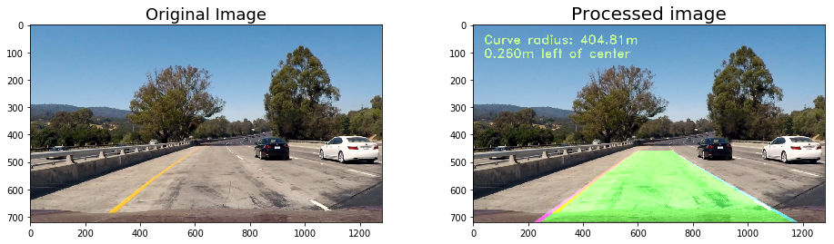
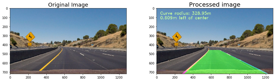
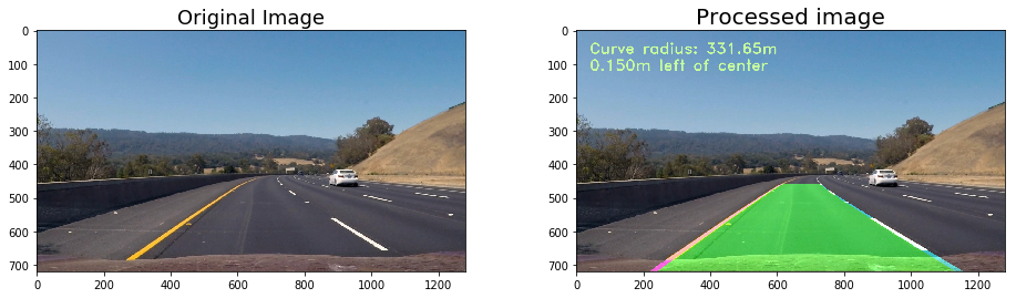
处理后结果如下:
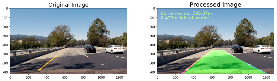
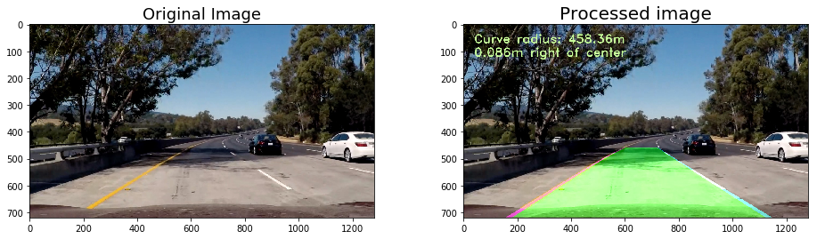
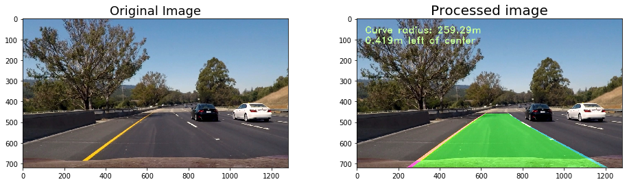
step7: Processing the video
处理视频数据,The finnal video can be found here
from moviepy.editor import VideoFileClip

output = 'project_video_output.mp4'
clip1 = VideoFileClip("project_video.mp4")
white_clip = clip1.fl_image(pipeline_final) #NOTE: this function expects color images!!
%time white_clip.write_videofile(output, audio=False)
总结
以上就是第二个Project的全部内容,主要就是摄像机的标定,投影变换,颜色通道,滑动窗口等技术,在计算机视觉领域得到了广泛应用。
本次处理的数据集较为简单,上面的pipeline在处理challenge video时会有问题,可能是光线过暗或是曲率过大的缘故,所以处理复杂道路场景下的视频数据是一项非常艰巨的任务,以这个车道线的提取为例,使用设定规则的方式提取车道线,虽然能够处理项目视频中的场景,但面对变化恶劣的场景仍然无能为力。
现阶段解决该问题的方法就是通过深度学习,拿足够多的标注数据去训练模型,才能尽可能的达到稳定的检测效果。