• Advanced Lane Finding
• Rubric Points
  • Step1:Camera Calibration
  • step2:Threshold binary image
  • step3:Apply a perspective transform to rectify binary image (“birds-eye view”)
  • step4:Lane detection and fit
    • 1. Taking a histogram along all the columns in the lower half of the image.
    • 2. Implementing Sliding Windows and Fit a Polynomial
    • 3. Searching around a previously detected line.
    • 4. Warping back to original perspective
  • step5: Drawing Curvature Radius and Distance from Center Data onto the Original Image
  • step6: Set the final pipeline
  • step7: Processing the video
• Discussion

Advanced Lane Finding

标签（空格分隔）： Self-Driving

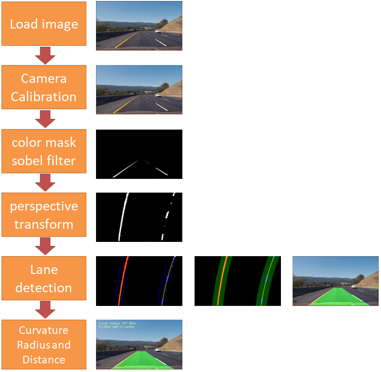
The goals / steps of this project are the following:

• Compute the camera calibration matrix and distortion coefficients given a set of chessboard images.
• Apply a distortion correction to raw images.
• Use color transforms, gradients, etc., to create a thresholded binary image.
• Apply a perspective transform to rectify binary image (“birds-eye view”).
• Detect lane pixels and fit to find the lane boundary.
• Determine the curvature of the lane and vehicle position with respect to center.
• Warp the detected lane boundaries back onto the original image.
• Output visual display of the lane boundaries and numerical estimation of lane curvature and vehicle position.

In this project, the camera calibration is performed by using the Chessboard Corners method.

Rubric Points

Step1:Camera Calibration

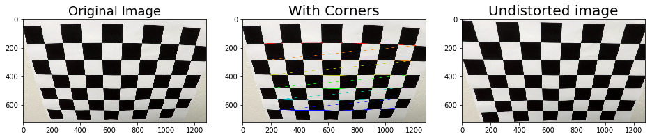
It can estimate the parameters of a lens and image sensor of an image or video camera. These parameters can be used to correct for lens distortion, measure the size of an object in world units, or determine the location of the camera in the scene. Opencv can claiberate camera to find out the parameters for reducing the distortion. There are basically two stages to calibration.

• First, we use a function in OpenCV called findChessboardCorners. We put all the images through this function, giving it our expected number of corners. For each successful call to this function, we then add the points we get back as well as a set of ‘normalized’ corners.
• With these in hand, we finally call calibrateCamera in OpenCV and get the matrix and distortion coefficients we will need to later call cv2.undistort to straighten images.

images = glob.glob('./camera_cal/calibration*.jpg')

def cal_undistort(img, objpoints, imgpoints):
    # Use cv2.calibrateCamera() and cv2.undistort()
    gray = cv2.cvtColor(img,cv2.COLOR_BGR2GRAY)
    ret, mtx, dist, rvecs, tvecs = cv2.calibrateCamera(objpoints, imgpoints, gray.shape[::-1], None, None)
    undist = cv2.undistort(img, mtx, dist, None, mtx)
    return undist

# Step through the list and search for chessboard corners
for fname in images:
    img = cv2.imread(fname)
    gray = cv2.cvtColor(img,cv2.COLOR_BGR2GRAY)

    # Find the chessboard corners
    ret, corners = cv2.findChessboardCorners(gray, (nx,ny),None)

    # If found, add object points, image points
    if ret == True:
        objpoints.append(objp)
        imgpoints.append(corners)
        
        img_corners = np.copy(img)
        img_corners = cv2.drawChessboardCorners(img_corners, (nx,ny), corners, ret)
        
        undist = cal_undistort(img, objpoints, imgpoints)
        ...

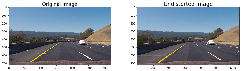
Next, I will use the calculated camera calibration matrix and distortion coefficients to remove distortion from the road images and output the undistorted images.

step2:Threshold binary image

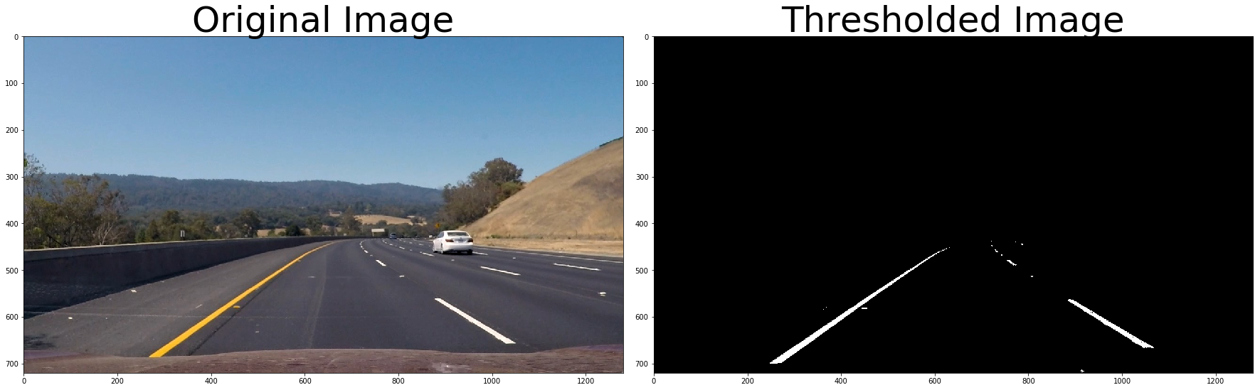
All code is contained in the get_thresholded_image() and abs_sobel_thresh() and dir_threshold()。

In order to detect lane lines in an image a binary threshold image is used. Any white image pixels are likely to be part of one of the two lane lines. All code required to create the binary threshold image is contained in function get_thresholded_image. That class uses a combination of the below elements:

• Sobel-x operators
• direction of the gradient
• R & G thresholds so that yellow lanes are detected well
• the S/L channel of the image (after converting it from BGR to HLS)

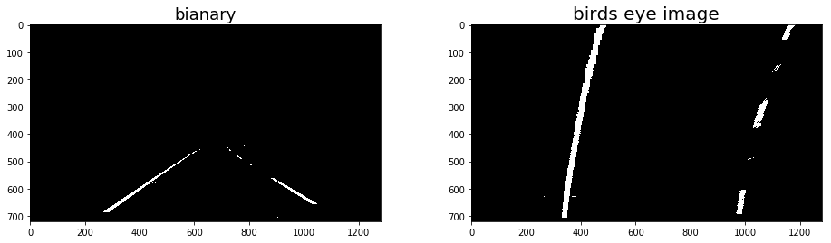
step3:Apply a perspective transform to rectify binary image (“birds-eye view”)

All code is contained in the birds_eye() 。

For my perspective transform, I specified 4 corners of a trapezoid (as src) in the undistorted original images and I specified the 4 corresponding corners of a rectangle (as dst) to which they are mapped in the perspective image. After inspecting an undistorted image, I specified the parameters as follows:

def birds_eye(img):
    img_size = (img.shape[1],img.shape[0])
    
    src = np.float32(
        [[585,460],
         [203,720],
         [695,460],
         [1127,720]]
    )
    dst = np.float32(
        [[320,0],
         [320,720],
         [960,0],
         [960,720]]
    )
    
    M = cv2.getPerspectiveTransform(src,dst)
    Minv = cv2.getPerspectiveTransform(dst, src)
    warped = cv2.warpPerspective(img,M,img_size,flags=cv2.INTER_LINEAR)
    
    return warped,M,Minv

Opencv provide two functions getPerspectiveTransform and warpPerspective to perform this task:

step4:Lane detection and fit

After applying calibration, thresholding, and a perspective transform to a road image, I have a binary image where the lane lines stand out clearly. However, I still need to decide explicitly which pixels are part of the lines and which belong to the left line and which belong to the right line.

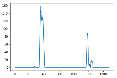
1. Taking a histogram along all the columns in the lower half of the image.

def hist(img):
    # Lane lines are likely to be mostly vertical nearest to the car
    bottom_half = img[img.shape[0]//2:,:]

    # Sum across image pixels vertically - make sure to set an `axis`
    # i.e. the highest areas of vertical lines should be larger values
    histogram = np.sum(bottom_half, axis=0)
    
    return histogram

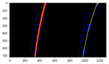
2. Implementing Sliding Windows and Fit a Polynomial

All code is contained in the fit_lines()。

• After splitting the image in half, the points in both halves with the highest number of pixels are assumed to be the starting points of the left and right lane line respectively。
• Using the two detected starting points for both lane lines, a sliding window approach is used to detect peaks in small areas around each starting point

After using the sliding window to detect lane line points starting at the bottom until the top of the image, second degree polynomials are fitted to both lane lines using numpy’s np.polyfit function. The two polynomials approximate the left and right lane lines respectively.

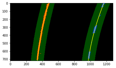
3. Searching around a previously detected line.

All code is contained in the fit_poly() and search_around_poly().

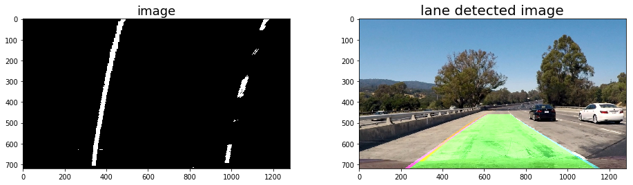
4. Warping back to original perspective

All code is contained in the draw_lane().

Once we know the position of lanes in birds-eye view, we use opencv function polyfill to draw a area in the image. Then, we warp back to original perspective.

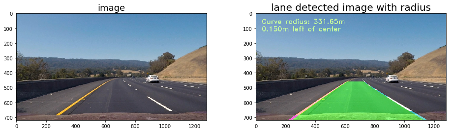
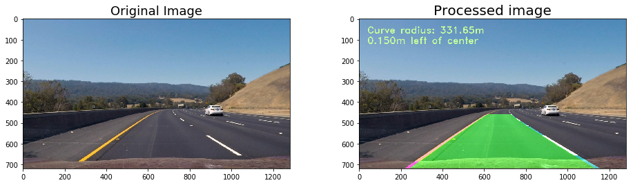
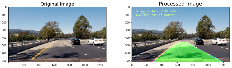
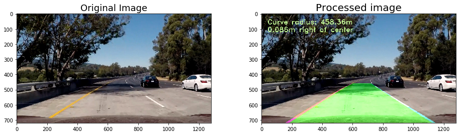
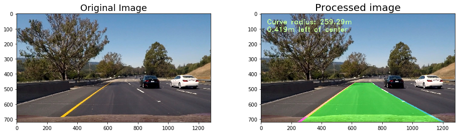
step5: Drawing Curvature Radius and Distance from Center Data onto the Original Image

All code is contained in the calc_curv_rad_and_center_dist() and draw_data().

I calculated the left and right radii of curvature using the formula r = (1 + (first_deriv)2)1.5 / abs(second_deriv):

# Fit new polynomials to x,y in world space
left_fit_cr = np.polyfit(lefty*ym_per_pix, leftx*xm_per_pix, 2)
right_fit_cr = np.polyfit(righty*ym_per_pix, rightx*xm_per_pix, 2)

# Calculate the new radii of curvature
left_curverad = ((1 + (2*left_fit_cr[0]*y_eval*ym_per_pix + left_fit_cr[1])**2)**1.5) / np.absolute(2*left_fit_cr[0])
right_curverad = ((1 + (2*right_fit_cr[0]*y_eval*ym_per_pix + right_fit_cr[1])**2)**1.5) / np.absolute(2*right_fit_cr[0])

I calculated the offset of the vehicle by the following code, the offset is image x midpoint - mean of l_fit and r_fit intercepts .

lane_center_position = (r_fit_x_int + l_fit_x_int) /2
center_dist = (car_position - lane_center_position) * xm_per_pix

Then draw the information to the Original Image。

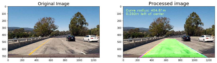
step6: Set the final pipeline

All code is contained in the pipeline_final().

Finally, I need a function to do all of the above tasks.

def pipeline_final(image):
    combined_binary = get_thresholded_image(image)
    warped,M,Minv = birds_eye(combined_binary)

    left_fit,right_fit = fit_lines(warped)
    result,left_fitx, right_fitx, ploty,left_lane_inds,right_lane_inds = search_around_poly(warped,left_fit,right_fit)
    rad_l, rad_r, d_center = calc_curv_rad_and_center_dist(warped, left_fit, right_fit, left_lane_inds, right_lane_inds)

    exampleImg_out1 = draw_lane(image, warped, left_fit, right_fit, Minv)
    exampleImg_out2 = draw_data(exampleImg_out1, (rad_l+rad_r)/2, d_center)
    
    return exampleImg_out2

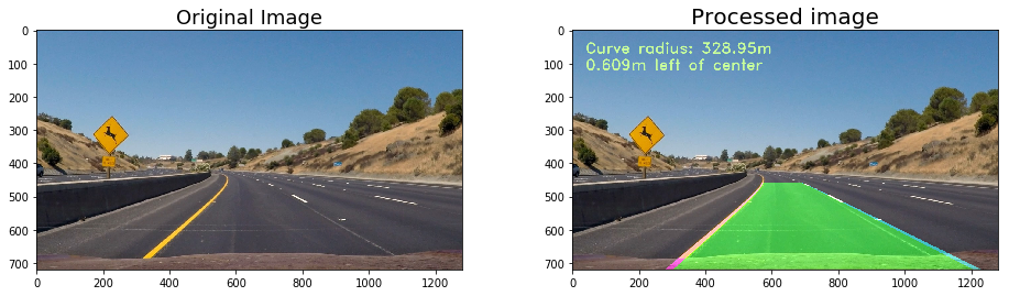
step7: Processing the video

The finnal video can be found here

from moviepy.editor import VideoFileClip

output = 'project_video_output.mp4'
clip1 = VideoFileClip("project_video.mp4")
white_clip = clip1.fl_image(pipeline_final) #NOTE: this function expects color images!!
%time white_clip.write_videofile(output, audio=False)

Discussion

• Places where pipeline is likely to fail

The pipeline doesn’t alright on the challenge video and the harder-challenge video.

• challenge video: maybe because the lane lines are much lighter than the first video.

• harder-challenge video: maybe because the lanes had large curvature, and as a result the lanes went outside the region of interest we chose for perspective transform.

• Plans to make pipeline more robust

I will improve the method of selection of lane line pixels so that even if the lane lines are light, they will still get picked up.