- 1. 回顾之前的机器学习
- 4. A Note on Deep Learning
- 12. Perceptrons 感知机
- 15. Perceptrons as Logical Operators
- 17. Perceptron Algorithm
- 20. Log-loss Error Function 误差函数(sigmoid函数)
- 21. Softmax
- 22. One-Hot Encoding
- 23. Maximum Likelihood 最大似然法
- 24. Maximizing Probabilities
- 25. Cross-Entropy 交叉熵
- 27. Multi-Class Cross Entropy
- 28. Logistic Regression 逻辑回归
- 29. Gradient Descent 梯度下降
- 30. Gradient Descent: The Code
- 31. Perceptron感知机 vs Gradient Descent梯度下降
- 35. Neural Network Architecture 神经网络结构
- 36. Feedforward 前向反馈
- 37. Multilayer Perceptrons 多层感知机
- 38. Backpropagation 反向传播
1. 回顾之前的机器学习
- 线性回归 Linear Regression

- 逻辑回归 Logistic Regression
上面的线性回归,预测一个连续的值,而逻辑回归用于预测一个离散的值,常用于分类问题,逻辑回归常用于自动驾驶中,比如判断一个物体是车还是行人,红灯还是绿灯等。

下面实际上是感知机的原理:

4. A Note on Deep Learning
接下来的学习中将设计神经网络的初级到中级,将使用TensorFlow和卷积神经网络,去从头构建一个神经网络:
- 神经网络简介(本章)
- MiniFlow
- TensorFlow入门
- 深度神经网络
- 卷积神经网络
12. Perceptrons 感知机
关于深度学习中的感知机,可以参考 here

上图就是一个感知机,w1,w2,wn是权重,b是偏置,第一个Linear function线性函数通过权重和偏置计算结果,传递给第二个节点即step function阶跃函数,通过阶跃函数判断。这里阶跃函数是激活函数的一种。
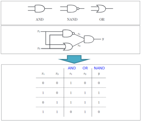
15. Perceptrons as Logical Operators
AND Perceptron:
下面是关于and感知机的实现,有些python技巧很实用
- outputs 是一个list,这个list内的元素也是list
num_wrong = len([output[4] for output in outputs if output[4] == 'No'])获取为No的个数
import pandas as pd

# TODO: Set weight1, weight2, and bias
weight1 = 1.0
weight2 = 1.0
bias = -1.5


# DON'T CHANGE ANYTHING BELOW
# Inputs and outputs
test_inputs = [(0, 0), (0, 1), (1, 0), (1, 1)]
correct_outputs = [False, False, False, True]
outputs = []

# Generate and check output
for test_input, correct_output in zip(test_inputs, correct_outputs):
    linear_combination = weight1 * test_input[0] + weight2 * test_input[1] + bias
    output = int(linear_combination >= 0)
    is_correct_string = 'Yes' if output == correct_output else 'No'
    outputs.append([test_input[0], test_input[1], linear_combination, output, is_correct_string])

# Print output
num_wrong = len([output[4] for output in outputs if output[4] == 'No'])
output_frame = pd.DataFrame(outputs, columns=['Input 1', '  Input 2', '  Linear Combination', '  Activation Output', '  Is Correct'])
if not num_wrong:
    print('Nice!  You got it all correct.\n')
else:
    print('You got {} wrong.  Keep trying!\n'.format(num_wrong))
print(output_frame.to_string(index=False))
输出如下:
Nice!  You got it all correct.

Input 1    Input 2    Linear Combination    Activation Output   Is Correct
      0          0                  -1.5                    0          Yes
      0          1                  -0.5                    0          Yes
      1          0                  -0.5                    0          Yes
      1          1                   0.5                    1          Yes
用相同的方式,可以实现OR,NOT感知机。
异或门XOR,可以用上述的组合来实现:
def XOR(x1,x2):
    s1 = NAND(x1,x2)
    s2 = OR(x1,x2)
    y = AND2(s1,s2)
    return y
参考下图:
17. Perceptron Algorithm

上面的实现代码如下:
import numpy as np
# Setting the random seed, feel free to change it and see different solutions.
np.random.seed(42)

def stepFunction(t):
    if t >= 0:
        return 1
    return 0

def prediction(X, W, b):
    return stepFunction((np.matmul(X,W)+b)[0])

# TODO: Fill in the code below to implement the perceptron trick.
# The function should receive as inputs the data X, the labels y,
# the weights W (as an array), and the bias b,
# update the weights and bias W, b, according to the perceptron algorithm,
# and return W and b.
def perceptronStep(X, y, W, b, learn_rate = 0.01):
    for i in range(len(X)):
        y_hat = prediction(X[i],W,b)
        if y[i]-y_hat == 1:
            W[0] += X[i][0]*learn_rate
            W[1] += X[i][1]*learn_rate
            b += learn_rate
        elif y[i]-y_hat == -1:
            W[0] -= X[i][0]*learn_rate
            W[1] -= X[i][1]*learn_rate
            b -= learn_rate
    return W, b


# This function runs the perceptron algorithm repeatedly on the dataset,
# and returns a few of the boundary lines obtained in the iterations,
# for plotting purposes.
# Feel free to play with the learning rate and the num_epochs,
# and see your results plotted below.
def trainPerceptronAlgorithm(X, y, learn_rate = 0.01, num_epochs = 25):
    x_min, x_max = min(X.T[0]), max(X.T[0])
    y_min, y_max = min(X.T[1]), max(X.T[1])
    W = np.array(np.random.rand(2,1))
    b = np.random.rand(1)[0] + x_max
    # These are the solution lines that get plotted below.
    boundary_lines = []
    for i in range(num_epochs):
        # In each epoch, we apply the perceptron step.
        W, b = perceptronStep(X, y, W, b, learn_rate)
        boundary_lines.append((-W[0]/W[1], -b/W[1]))
    return boundary_lines

上面函数的调用构成如下图:

- trainPerceptronAlgorithm(),根据指定的学习率和迭代次数,计算调整后的权值和偏置。
- perceptronStep(),根据指定的学习率,以及预测结果及标签,调整权值和偏置。
- y[i] = 1 (标签为正),y_hat = 0(预测为负),用加法调整权值和偏置
- y[i] = 0 (标签为负),y_hat = 1(预测为正),用减法法调整权值和偏置
- prediction(),调用激活函数(阶跃函数),得到最终的输出,即预测结果
- stepFunction(),最后的激活函数-阶跃函数
调整学习率和迭代次数结果如下:

可以看出,如何设定学习率和迭代次数,对最终结果有直接影响:
- 学习率过大(0.1),会导致每一步的步幅过大,难以得到正确的结果。
- 迭代次数过少(5),会导致还没有达到最好效果就结束了;迭代次数过大(100),会做无用功。
20. Log-loss Error Function 误差函数(sigmoid函数)
参考损失函数(lost function) 关于sigmoid函数,参考2.2 sigmoid函数
一个误差函数要保证连续,可求导()两个条件,即:
- The error function should be differentiable.
- The error function should be continuous.
基于上面损失函数的规律,所以激活函数要有连续可到的特性,如下图,将激活函数从阶跃函数(离散)变为了sigmoid函数(连续),输出结果从是否被录取,变成了录取的概率:

参考下图:

- 连续可导的激活函数sigmoid函数,在x无穷大时,结果趋于1,x为无穷小时,结果趋于0。
代码实现如下:
def sigmoid(x):
    return 1 / (1 + np.exp(-x))
练习题:
The sigmoid function is defined as sigmoid(x) = 1/(1+e-x). If the score is defined by 4x1 + 5x2 - 9 = score, then which of the following points has exactly a 50% probability of being blue or red? (Choose all that are correct.)
答案是 (1,1)和(-4,5),即只要得到了score为0,则最终的sigmoid函数结果为0.5.

21. Softmax
上面介绍了阶跃函数和sigmoid函数,分别表示是否录取,或是录取的概率,那如果输出有多个结果呢,比如录取的是北大,还是清华,或是复旦,这里要用到Softmax函数。
def softmax(L):
    expL = np.exp(L)
    sumExpL = sum(expL)
    result = []
    for i in expL:
        result.append(i*1.0/sumExpL)
    return result

22. One-Hot Encoding
这种方式叫One-hot Encoding,在处理数据时经常使用。

如上图中,针对每一种结果,都有一个标签,这个标签是一个list,这个list中包含的元素个数,与结果的总数相同,然后在对应的位置设为1.
在另一个手写数字识别中也是这样做的,有0-9共10种测试结果,比如0的标签为[1,0,0,0,0,0,0,0,0]。
23. Maximum Likelihood 最大似然法
如下图,分别是两种模型的预测结果,通过两种模型结果中,各个预测值的概率乘积总和,判断哪种模型更加准确,这种方式叫做最大似然法:

24. Maximizing Probabilities
We will learn how to maximize a probability, using some math. Nothing more than high school math, so get ready for a trip down memory lane!
参考上面的图,如果将所有概率乘起来的话,其结果将是一个很小的数,我们需要将其乘积转换为和的形式,通过log函数,可以将乘积变成求和的形式,如下:
log(p1*p2*p3*p4..*pn*) = logp1 + logp2 + logp3 + .. logpn
25. Cross-Entropy 交叉熵
上面将乘积形式转换后的求和形式,叫做交叉熵。模型越准确,交叉熵越小,参考下图:

如下用示例解释交叉熵:

(1,1,0)表示标签,即前面两个有礼物,后一个无礼物;(0.8,0.7,0.1)表示出现这种标签的概率
用代码实现如下:
import numpy as np

def cross_entropy(Y, P):
    Y = np.float_(Y)
    P = np.float_(P)
    return -np.sum(Y * np.log(P) + (1 - Y) * np.log(1 - P))
27. Multi-Class Cross Entropy
上面的结果中只有是和否,如果结果是多个的情况下,用如下的交叉熵公式:

28. Logistic Regression 逻辑回归
逻辑回归大致步骤如下:
- 准备数据
- 选取一个随机模型
- 计算误差
- 最小化误差,优化模型
下面分别是二元分类和多元分类问题的误差函数:

通过梯度下降的方法,找到其对应的最小误差:

梯度的计算方法,可以参考4.1 梯度法
在某点的上方和下方(极小处),分别取一个点,求这两个点之间的斜率。
29. Gradient Descent 梯度下降
参考4.1 梯度法

参考上图,每次通过学习率和导数去调整权重和偏置,得到更好的权重和偏置。
梯度计算公式推导:
上面几个部分中,我们了解到要最小化损失函数,就要计算其导数,下面实际推导一下误差函数的导数。
无语了,全是微积分的推导,这些基本公式都忘了,不理解…微积分得从头补起来,不然真是空中楼阁。

30. Gradient Descent: The Code
权重的更新值为:Δwi=α∗δ∗xi,其中α是学习率,δ是误差项。
相关代码如下:
# Defining the sigmoid function for activations
def sigmoid(x):
    return 1/(1+np.exp(-x))

# Derivative of the sigmoid function
def sigmoid_prime(x):
    return sigmoid(x) * (1 - sigmoid(x))

# Input data
x = np.array([0.1, 0.3])
# Target
y = 0.2
# Input to output weights
weights = np.array([-0.8, 0.5])

# The learning rate, eta in the weight step equation
learnrate = 0.5

# The neural network output (y-hat)
nn_output = sigmoid(x[0]*weights[0] + x[1]*weights[1])
# or nn_output = sigmoid(np.dot(x, weights))

# output error (y - y-hat)
error = y - nn_output

# error term (lowercase delta)
error_term = error * sigmoid_prime(np.dot(x,weights))

# Gradient descent step
del_w = [ learnrate * error_term * x[0],
                 learnrate * error_term * x[1]]
# or del_w = learnrate * error_term * x
- error_term是误差项δ,通过
error * sigmoid_prime(np.dot(x,weights))计算得到。 - del_w是权重的更新值。
练习的代码:
import numpy as np

def sigmoid(x):
    """
    Calculate sigmoid
    """
    return 1/(1+np.exp(-x))

def sigmoid_prime(x):
    return sigmoid(x) * (1 - sigmoid(x))

learnrate = 0.5
x = np.array([1, 2])
y = np.array(0.5)

# Initial weights
w = np.array([0.5, -0.5])

# Calculate one gradient descent step for each weight
# TODO: Calculate output of neural network
nn_output = sigmoid(np.dot(x, w))
# nn_output = sigmoid(x[0]*w[0] + x[1]*w[1])

# TODO: Calculate error of neural network
error = y - nn_output

# TODO: Calculate change in weights
del_w = learnrate * error * nn_output * (1 - nn_output) * x

print('Neural Network output:')
print(nn_output)
print('Amount of Error:')
print(error)
print('Change in Weights:')
print(del_w)
输出结果如下:
Neural Network output:
0.3775406687981454
Amount of Error:
0.1224593312018546
Change in Weights:
[0.0143892 0.0287784]

Nice job!  That's right!
31. Perceptron感知机 vs Gradient Descent梯度下降
感知机和梯度下降参考如下:
下图是感知机和梯度下降的区别:
- 感知机只有在分类错误时,才去调整权重,而梯度下降会不断调整权重。
- 感知机使用的是阶跃函数,预测值y和标签的y,要么是1,要么是0;而梯度下降是一个概率值在0-1之间。
- 感知机的权值调整,可以看做是梯度下降的一种特殊case,感知机只有两种情况,wi + axi和wi - axi。

35. Neural Network Architecture 神经网络结构
35.1 简单结构的神经网络
构建一个非线性的神经网络结构:
- 通过两个线性模型的叠加求和,最终使用sigmoid激活函数,得到新的非线性模型,如下图所示:

- 通过给线性模型添加权重和偏置,得到更复杂的新模型:

将结构图修改如下,就有点像神经网络的样子了:

练习:
Based on the above video, let’s define the combination of two new perceptrons as w10.4 + w20.6 + b. Which of the following values for the weights and the bias would result in the final probability of the point to be 0.88?
w1:2,w2:6;b:-2 w1:3,w2:5;b:-2.2 w1:5,w2:4;b:-3
将上面三个选项,代入上面的线性模型,分别得到2.4,2,1.4 三个值,然后代入sigmoid函数求解,代码如下:
def sigmoid(x):
    return 1 / (1 + np.exp(-x))

print(sigmoid(2.4))
print(sigmoid(2))
print(sigmoid(1.4))
得到结果为如下,所以第二个选项正确:
0.916827303506
0.880797077978
0.802183888559
35.2 Multiple layers 多层结构的神经网络
上面的神经网络比较简单,如下的网络更加复杂:
- 给输入层,隐藏层,输出层添加更多的节点
- 添加更多的隐藏层
如下图:


多元分类:
一个输入,最终有多个输出,输出每个种类出现的概率,或是softmax函数值:

softmax函数代码如下:
# Softmax函数
def softmax(a):
    exp_a = np.exp(a)
    sum_exp_a = np.sum(exp_a)
    y = exp_a / sum_exp_a

    return y
参考手写图片的数字识别处理神经网络的推理处理 输出层有10个结果,分别代码是0-9的概率或是其他的指标值。
36. Feedforward 前向反馈
通过权重/偏置/激活函数,最终计算出预测值,这就是神经网络的前向反馈。

Error Function 误差函数:

37. Multilayer Perceptrons 多层感知机
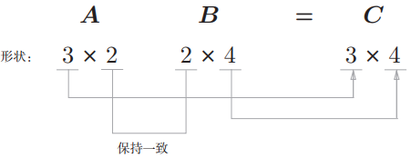
下面介绍多层感知机神经网络中的数学知识,下面将使用到vector向量和矩阵matrice。
现在我们处理的这个感知机,有复数个input,复数个隐藏层的node,在这两者之间的权重,要满足:
- Wij,i表示行数,j表示列数,i与input的元素个数相同,j与隐藏层个数相同。

参考如下代码:
# Number of records and input units
n_records, n_inputs = features.shape
# Number of hidden units
n_hidden = 2
weights_input_to_hidden = np.random.normal(0, n_inputs**-0.5, size=(n_inputs, n_hidden))
上面生成了一个input层到hidden层的权重矩阵,hidden层上的各个unit的计算方式为:

代码如下:
hidden_inputs = np.dot(inputs, weights_input_to_hidden)

通过上面的图可以很好的理解,为什么权重矩阵的行数与input的列数一样,权重矩阵的列数与隐藏层的列数一样。
矩阵的翻转:
matrix = [[2,3,4],[5,6,7]]
matrix = np.array(matrix, ndmin=2)
print(matrix)
print("--------------")
print(matrix.T)
如下:
matrix = [[2,3,4],[5,6,7]]
matrix = np.array(matrix, ndmin=2)
print(matrix,"===",matrix.shape)
print("--------------")
print(matrix.T,"===",matrix.T.shape)
翻转后结果如下:
[[2 3 4]
 [5 6 7]] === (2, 3)
--------------
[[2 5]
 [3 6]
 [4 7]] === (3, 2)
matrix = [5,6,7]
matrix = np.array(matrix)
print(matrix,"===",matrix.shape)
print("--------------")
print(matrix.T,"===",matrix.T.shape)
如果是一维的,结果不变:
[5 6 7] === (3,)
--------------
[5 6 7] === (3,)
Programming quiz:
Below, you’ll implement a forward pass through a 4x3x2 network, with sigmoid activation functions for both layers.
Things to do:
- Calculate the input to the hidden layer.
- Calculate the hidden layer output.
- Calculate the input to the output layer.
- Calculate the output of the network.
代码:
import numpy as np

def sigmoid(x):
    """
    Calculate sigmoid
    """
    return 1/(1+np.exp(-x))

# Network size
N_input = 4
N_hidden = 3
N_output = 2

np.random.seed(42)
# Make some fake data
X = np.random.randn(4)

weights_input_to_hidden = np.random.normal(0, scale=0.1, size=(N_input, N_hidden))
weights_hidden_to_output = np.random.normal(0, scale=0.1, size=(N_hidden, N_output))


# TODO: Make a forward pass through the network

hidden_layer_in = np.dot(X, weights_input_to_hidden)
hidden_layer_out = sigmoid(hidden_layer_in)

print('Hidden-layer Output:')
print(hidden_layer_out)

output_layer_in = np.dot(hidden_layer_out, weights_hidden_to_output)
output_layer_out = sigmoid(output_layer_in)

print('Output-layer Output:')
print(output_layer_out)
Hidden-layer Output:
[0.41492192 0.42604313 0.5002434 ]
Output-layer Output:
[0.49815196 0.48539772]

Nice job!  That's right!

38. Backpropagation 反向传播
现在该轮到我们实际的训练一个神经网络,在这里我们使用一种叫反向传播的方式,简而言之,反向传播包括如下的几点:
- 进行正向反馈操作
- 将模型输出与期望输出(标签)进行对比
- 计算误差
- 使用反向传播将误差反映到权重上
- 用这个去更新权重,得到一个更好的模型
- 循环上述步骤,至到得到一个满意的模型
反向传播是深度学习的基础,TensorFlow和其他一些库虽说已经将其封装完好,但是自己还是要理解其算法。
可以参考误差反向传播