- 0. 总结:
- 6. Intuition
- 7. Filters 滤波器
- 8. Feature Map Sizes
- 9. Convolutions continued
- 10. Parameters
- 11. Quiz: Convolution Output Shape
- 13. Quiz: Number of Parameters
- 15. Quiz: Parameter Sharing
- 17. Visualizing CNNs
- 18. TensorFlow Convolution Layer
- 19. Explore The Design Space
- 20. TensorFlow Max Pooling
- 23. Quiz: Pooling Mechanics
- 29. 1x1 Convolutions
- 31. Convolutional Network in TensorFlow
- 32. TensorFlow Convolutional Layer Workspaces
- 34. TensorFlow Pooling Layer Workspaces
- 36. Lab: LeNet in TensorFlow
- 37. LeNet Lab Workspace
- 37. Lab代码解析
- 38. CNNs - Additional Resources
本章参考深度学习入门-07-卷积神经网络
0. 总结:
本章非常重要,udacity的CNN讲解得太坑爹了,太概略,不另外看书的话简直如听天书.(不过这本不是udacity的长处,不怪他) 这里除了讲解CNN的概念外,主要讲解了如何利用TensorFlow实现CNN,尤其是LeNet。
- 滤波器,本质上就是权重,通过权重共享,减少参数,缩小output的size。
- 如何根据input/滤波器(步长,size),偏置等计算output的size和depth。
- padding在TensorFlow中分为Same和Valid,其计算公式,与一般的概念上稍有差异,需要注意。
- 经过卷积层处理后,最终都要经过全连接层(Full connected layer),最后提供给分类器。
- CNN各层的可视化,可以看到每一层都能抽象出一些特征,越往后其特征就越明显。
- 池化处理是CNN中减少input数量的方式,有Max池化以及平均值池化等方式。
- 最终通过实例代码,解释了上述的概念在TensorFlow中如何实现。
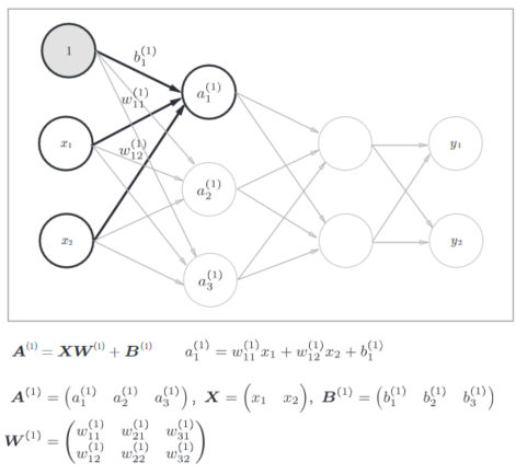
6. Intuition
一个CNN会有很多层,每个层上会有不同的特征,这些层上的特征都是CNN自身学习得到的,不需要人为去指定各个层的特征。
7. Filters 滤波器
CNN神经网络的第一步,就是将图片分割成更小的块,这个分割的过程通过滤波器完成。
这个分割过程,在这里有详细讲解卷积运算
将滤波器应用在输入数据即图片上,按照步长(stride)进行移动,不断进行矩阵乘积运算,得到新的输出,一般来说增加步长会导致model的size变小,减少了一个layer上的神经元数量,最终导致精度降低。
Filter Depth(滤波器深度):
一般来说滤波器不止一个,不同的滤波器应用到不同的通道上(R/G/B),具体可以参考3维数据的卷积运算。
8. Feature Map Sizes

- input depth 表示输入数据有3个通道
- output depth 表示输出数据有8个通道,说明滤波器是个四维的数据,size为(8,3,3,3),表示意义为(FN滤波器个数,C通道,FH高,FW宽)
- Padding是same,表示输入数据会有填充,以保证输出数据的高宽,与输入数据一样,所以,padding为same,步幅stride是1时,三个值分别是(28,28,8)
- Padding是valid,表示没有填充,滤波器移动时不超过边界,根据下面的公式计算,如果步长stride为1,则结果为(26,26,8);步长为2,则结果为(13,13,8)。

另外,多个滤波器的卷积元素,参考下图:

Same padding / valid padding:
Same padding表示会对输入数据进行填充,使得输出数据与输入数据有相同的高和宽,而valid padding是不会填充,移动时不会超过边界。

9. Convolutions continued

卷积层计算完毕后,需要将其变换成全连接层(Full connected layer),然后训练分类器。
如何变换成全连接层,可以参考基于im2col的展开
A “Fully Connected” layer is a standard, non convolutional layer, where all inputs are connected to all output neurons. This is also referred to as a “dense” layer, and is what we used in the previous two lessons.
10. Parameters
一般来说,我们在识别的时候,不需要理会识别对象所在的问题,不管是在左上或是右下,在我们眼中都是该对象。 我们希望CNN也有相同的处理能力(平移不变性translation invariance)。
如之前描述的,图片上给定patch的分类,由该patch对应的权重和偏置所决定。 所以,如果希望左上角的猫,和右下角的猫,都能被CNN识别为猫,那他们需要相同的权重和偏置。
实际上上面解释的,可以参考卷积层,详细的讲解了步长,填充,以及卷积运算的步骤。
Dimensionality 维度:
1. input layer has a width of W and a height of H
2. our convolutional layer has a filter size F
3. the number of filters : K
4. stride : S
5. padding : P
- the following formula gives us the width of the next layer: W_out =[ (W−F+2P)/S] + 1
- The output height would be H_out = [(H-F+2P)/S] + 1
- the output depth would be equal to the number of filters D_out = K
- The output volume would be
W_out * H_out * D_out
11. Quiz: Convolution Output Shape
- We have an input of shape 32x32x3 (HxWxD)
- 20 filters of shape 8x8x3 (HxWxD)
- A stride of 2 for both the height and width (S)
- With padding of size 1 (P)
根据下面的公式:
new_height = (input_height - filter_height + 2 * P)/S + 1
new_width = (input_width - filter_width + 2 * P)/S + 1
计算出output的shape为:14x14x20.
上面的实现过程用TensorFlow代码如下:
input = tf.placeholder(tf.float32, (None, 32, 32, 3))
filter_weights = tf.Variable(tf.truncated_normal((8, 8, 3, 20))) # (height, width, input_depth, output_depth)
filter_bias = tf.Variable(tf.zeros(20))
strides = [1, 2, 2, 1] # (batch, height, width, depth)
padding = 'SAME'
conv = tf.nn.conv2d(input, filter_weights, strides, padding) + filter_bias
通过上面的代码计算出来的conv的形状为[1,16,16,20],并不与我们预期的[1,14,14,20]相同,这是因为TensorFlow中的SAME和VALID,与之前讲解的不同。
如果将SAME修改为VALID,最终conv的shape为[1,13,13,20]。
TensorFlow中关于SAME和VALID下output的shape计算方式如下:
SAME Padding:
out_height = ceil(float(in_height) / float(strides[1]))
out_width = ceil(float(in_width) / float(strides[2]))
VALID Padding:
out_height = ceil(float(in_height - filter_height + 1) / float(strides[1]))
out_width = ceil(float(in_width - filter_width + 1) / float(strides[2]))
13. Quiz: Number of Parameters
- We have an input of shape 32x32x3 (HxWxD)
- 20 filters of shape 8x8x3 (HxWxD)
- A stride of 2 for both the height and width (S)
- With padding of size 1 (P)
output layer: 14x14x20 (HxWxD)
Hint:
Without parameter sharing, each neuron in the output layer must connect to each neuron in the filter. In addition, each neuron in the output layer must also connect to a single bias neuron.
参考下面的图,可以计算得到,如果没有权重共享的话,将会有(8 * 8 * 3 + 1) * (14 * 14 * 20) = 756560个参数。
8 * 8 * 3是权重的个数,1是表示bias个数,右边的14 * 14 * 20是连接着的输出层的神经元数量。
15. Quiz: Parameter Sharing
同样是上面的条件,如果有权值共享的话,那么参数的个数是多少呢?
- We have an input of shape 32x32x3 (HxWxD)
- 20 filters of shape 8x8x3 (HxWxD)
- A stride of 2 for both the height and width (S)
- With padding of size 1 (P)
output layer: 14x14x20 (HxWxD)
Hint:
With parameter sharing, each neuron in an output channel shares its weights with every other neuron in that channel. So the number of parameters is equal to the number of neurons in the filter, plus a bias neuron, all multiplied by the number of channels in the output layer.
结果是:
(8 * 8 * 3 + 1) * 20 = 3840 + 20 = 3860
3840是权重,20是偏置,在权重共享中,我们在一个通道上使用同一个filter即权重,可以参考下图。

17. Visualizing CNNs
CNN的可视化,对应CNN的可视化
下面的例子来自于ImageNet中的识别结果,列举Layer1-Layer5的识别出的特征:
Layer1:

Layer2:

Layer3:

Layer5:

可以看到,随着层次的加深,其特征也越来越明显。
18. TensorFlow Convolution Layer
下面看看TensorFlow中如何实施CNN,可以使用 tf.nn.conv2d() and tf.nn.bias_add()去生成卷积层:
# Output depth
k_output = 64

# Image Properties
image_width = 10
image_height = 10
color_channels = 3

# Convolution filter
filter_size_width = 5
filter_size_height = 5

# Input/Image
input = tf.placeholder(
    tf.float32,
    shape=[None, image_height, image_width, color_channels])

# Weight and bias
weight = tf.Variable(tf.truncated_normal(
    [filter_size_height, filter_size_width, color_channels, k_output]))
bias = tf.Variable(tf.zeros(k_output))

# Apply Convolution
conv_layer = tf.nn.conv2d(input, weight, strides=[1, 2, 2, 1], padding='SAME')
# Add bias
conv_layer = tf.nn.bias_add(conv_layer, bias)
# Apply activation function
conv_layer = tf.nn.relu(conv_layer)
tf.nn.conv2d(): 利用滤波器(权重)和步长,以及填充方式作为input,生成卷积层strides=[1, 2, 2, 1]: strides: A list of ints. 1-D tensor of length 4. The stride of the sliding window for each dimension of input. For the most common case of the same horizontal and vertices strides, strides = [1, stride, stride, 1].input: Given an input tensor of shape [batch, in_height, in_width, in_channels]tf.nn.bias_add():adds a 1-d bias to the last dimension in a matrix.
19. Explore The Design Space
主要介绍了池化层,详细可以参考池化层
20. TensorFlow Max Pooling

如上图,是Max池化,以2*2滤波器和2的步长,对input进行处理,得到右边的结果。
通过池化处理:能减少input的数据量,将最主要的值保留下来。
TensorFlow中使用tf.nn.max_pool()函数实现卷积层的池化:
...
conv_layer = tf.nn.conv2d(input, weight, strides=[1, 2, 2, 1], padding='SAME')
conv_layer = tf.nn.bias_add(conv_layer, bias)
conv_layer = tf.nn.relu(conv_layer)
# Apply Max Pooling
conv_layer = tf.nn.max_pool(
    conv_layer,
    ksize=[1, 2, 2, 1],
    strides=[1, 2, 2, 1],
    padding='SAME')
- ksize:parameter as the size of the filter
- strides:parameter as the length of the stride
The ksize and strides parameters are structured as 4-element lists, with each element corresponding to a dimension of the input tensor ([batch, height, width, channels]). For both ksize and strides, the batch and channel dimensions are typically set to 1.
A pooling layer is generally used to:
- Decrease the size of the output
- Prevent overfitting
Reducing overfitting is a consequence of the reducing the output size, which in turn, reduces the number of parameters in future layers.
但是最近,池化技术逐渐失宠,主要是:
- Dropout能提供更好的正则化。(Dropout是一种在学习的过程中随机删除神经元的方法,训练时,随机选出隐藏层的神经元,然后将其删除,被删除的神经元不再进行信号的传递。)
- 池化导致了信息丢失。
23. Quiz: Pooling Mechanics
关于池化层和input层的定义如下:
- We have an input of shape 4x4x5 (HxWxD)
- Filter of shape 2x2 (HxW)
- A stride of 2 for both the height and width (S)
最终处理后的结果公式如下:
new_height = (input_height - filter_height)/S + 1
new_width = (input_width - filter_width)/S + 1

output is 2x2x5,相应的代码如下:
input = tf.placeholder(tf.float32, (None, 4, 4, 5))
filter_shape = [1, 2, 2, 1]
strides = [1, 2, 2, 1]
padding = 'VALID'
pool = tf.nn.max_pool(input, filter_shape, strides, padding)
最后输出的pool应该是[1, 2, 2, 5]。
29. 1x1 Convolutions
udacity这个视频讲的啥啊,…无语了,完全没懂,看看吴恩达讲的视频Neural Networks - Networks in Networks and 1x1 Convolutions
31. Convolutional Network in TensorFlow
31.1 示例代码
from tensorflow.examples.tutorials.mnist import input_data
mnist = input_data.read_data_sets(".", one_hot=True, reshape=False)

import tensorflow as tf

# Parameters
learning_rate = 0.00001
epochs = 10
batch_size = 128

# Number of samples to calculate validation and accuracy
# Decrease this if you're running out of memory to calculate accuracy
test_valid_size = 256

# Network Parameters
n_classes = 10  # MNIST total classes (0-9 digits)
dropout = 0.75  # Dropout, probability to keep units


# Store layers weight & bias
weights = {
    'wc1': tf.Variable(tf.random_normal([5, 5, 1, 32])),
    'wc2': tf.Variable(tf.random_normal([5, 5, 32, 64])),
    'wd1': tf.Variable(tf.random_normal([7*7*64, 1024])),
    'out': tf.Variable(tf.random_normal([1024, n_classes]))}

biases = {
    'bc1': tf.Variable(tf.random_normal([32])),
    'bc2': tf.Variable(tf.random_normal([64])),
    'bd1': tf.Variable(tf.random_normal([1024])),
    'out': tf.Variable(tf.random_normal([n_classes]))}


def conv2d(x, W, b, strides=1):
    x = tf.nn.conv2d(x, W, strides=[1, strides, strides, 1], padding='SAME')
    x = tf.nn.bias_add(x, b)
    return tf.nn.relu(x)

def maxpool2d(x, k=2):
    return tf.nn.max_pool(x, ksize=[1, k, k, 1], strides=[1, k, k, 1], padding='SAME')

def conv_net(x, weights, biases, dropout):
    # Layer 1 - 28*28*1 to 14*14*32
    conv1 = conv2d(x, weights['wc1'], biases['bc1'])
    conv1 = maxpool2d(conv1, k=2)

    # Layer 2 - 14*14*32 to 7*7*64
    conv2 = conv2d(conv1, weights['wc2'], biases['bc2'])
    conv2 = maxpool2d(conv2, k=2)

    # Fully connected layer - 7*7*64 to 1024
    fc1 = tf.reshape(conv2, [-1, weights['wd1'].get_shape().as_list()[0]])
    fc1 = tf.add(tf.matmul(fc1, weights['wd1']), biases['bd1'])
    fc1 = tf.nn.relu(fc1)
    fc1 = tf.nn.dropout(fc1, dropout)

    # Output Layer - class prediction - 1024 to 10
    out = tf.add(tf.matmul(fc1, weights['out']), biases['out'])
    return out

# tf Graph input
x = tf.placeholder(tf.float32, [None, 28, 28, 1])
y = tf.placeholder(tf.float32, [None, n_classes])
keep_prob = tf.placeholder(tf.float32)

# Model
logits = conv_net(x, weights, biases, keep_prob)

# Define loss and optimizer
cost = tf.reduce_mean(tf.nn.softmax_cross_entropy_with_logits(logits=logits, labels=y))
optimizer = tf.train.GradientDescentOptimizer(learning_rate=learning_rate).minimize(cost)

# Accuracy
correct_pred = tf.equal(tf.argmax(logits, 1), tf.argmax(y, 1))
accuracy = tf.reduce_mean(tf.cast(correct_pred, tf.float32))

# Initializing the variables
init = tf.global_variables_initializer()

# Launch the graph
with tf.Session() as sess:
    sess.run(init)

    for epoch in range(epochs):
        for batch in range(mnist.train.num_examples//batch_size):
            batch_x, batch_y = mnist.train.next_batch(batch_size)
            sess.run(optimizer, feed_dict={x: batch_x, y: batch_y, keep_prob: dropout})

            # Calculate batch loss and accuracy
            loss = sess.run(cost, feed_dict={x: batch_x, y: batch_y, keep_prob: 1.})
            valid_acc = sess.run(accuracy, feed_dict={
                x: mnist.validation.images[:test_valid_size],
                y: mnist.validation.labels[:test_valid_size],
                keep_prob: 1.})

            print('Epoch {:>2}, Batch {:>3} - Loss: {:>10.4f} Validation Accuracy: {:.6f}'.format(
                epoch + 1,
                batch + 1,
                loss,
                valid_acc))

    # Calculate Test Accuracy
    test_acc = sess.run(accuracy, feed_dict={
        x: mnist.test.images[:test_valid_size],
        y: mnist.test.labels[:test_valid_size],
        keep_prob: 1.})
    print('Testing Accuracy: {}'.format(test_acc))
31.2 代码分析:
导入数据集并定义各种超参数:
from tensorflow.examples.tutorials.mnist import input_data
mnist = input_data.read_data_sets(".", one_hot=True, reshape=False)

import tensorflow as tf

# Parameters
learning_rate = 0.00001
epochs = 10
batch_size = 128

# Number of samples to calculate validation and accuracy
# Decrease this if you're running out of memory to calculate accuracy
test_valid_size = 256

# Network Parameters
n_classes = 10  # MNIST total classes (0-9 digits)
dropout = 0.75  # Dropout, probability to keep units
Weights and Biases:
# Store layers weight & bias
weights = {
    'wc1': tf.Variable(tf.random_normal([5, 5, 1, 32])),
    'wc2': tf.Variable(tf.random_normal([5, 5, 32, 64])),
    'wd1': tf.Variable(tf.random_normal([7*7*64, 1024])),
    'out': tf.Variable(tf.random_normal([1024, n_classes]))}

biases = {
    'bc1': tf.Variable(tf.random_normal([32])),
    'bc2': tf.Variable(tf.random_normal([64])),
    'bd1': tf.Variable(tf.random_normal([1024])),
    'out': tf.Variable(tf.random_normal([n_classes]))}
Convolutions:
In TensorFlow, this is all done using tf.nn.conv2d() and tf.nn.bias_add().
def conv2d(x, W, b, strides=1):
    x = tf.nn.conv2d(x, W, strides=[1, strides, strides, 1], padding='SAME')
    x = tf.nn.bias_add(x, b)
    return tf.nn.relu(x)
Max Pooling:

def maxpool2d(x, k=2):
    return tf.nn.max_pool(
        x,
        ksize=[1, k, k, 1],
        strides=[1, k, k, 1],
        padding='SAME')
Model:

下面的代码中创建了三层网络,下面代码的注释中解释了每一层中神经元维度的变化,Layer1中,先通过conv2d将28×28×1转换成28×28×32,再应用max pool,将其转换为14×14×32。(32应该表示是通道,将一副图分割了32个通道)
def conv_net(x, weights, biases, dropout):
    # Layer 1 - 28*28*1 to 14*14*32
    conv1 = conv2d(x, weights['wc1'], biases['bc1'])
    conv1 = maxpool2d(conv1, k=2)

    # Layer 2 - 14*14*32 to 7*7*64
    conv2 = conv2d(conv1, weights['wc2'], biases['bc2'])
    conv2 = maxpool2d(conv2, k=2)

    # Fully connected layer - 7*7*64 to 1024
    fc1 = tf.reshape(conv2, [-1, weights['wd1'].get_shape().as_list()[0]])
    fc1 = tf.add(tf.matmul(fc1, weights['wd1']), biases['bd1'])
    fc1 = tf.nn.relu(fc1)
    fc1 = tf.nn.dropout(fc1, dropout)

    # Output Layer - class prediction - 1024 to 10
    out = tf.add(tf.matmul(fc1, weights['out']), biases['out'])
    return out
Session:
# tf Graph input
x = tf.placeholder(tf.float32, [None, 28, 28, 1])
y = tf.placeholder(tf.float32, [None, n_classes])
keep_prob = tf.placeholder(tf.float32)

# Model
logits = conv_net(x, weights, biases, keep_prob)

# Define loss and optimizer
cost = tf.reduce_mean(\
    tf.nn.softmax_cross_entropy_with_logits(logits=logits, labels=y))
optimizer = tf.train.GradientDescentOptimizer(learning_rate=learning_rate)\
    .minimize(cost)

# Accuracy
correct_pred = tf.equal(tf.argmax(logits, 1), tf.argmax(y, 1))
accuracy = tf.reduce_mean(tf.cast(correct_pred, tf.float32))

# Initializing the variables
init = tf. global_variables_initializer()

# Launch the graph
with tf.Session() as sess:
    sess.run(init)

    for epoch in range(epochs):
        for batch in range(mnist.train.num_examples//batch_size):
            batch_x, batch_y = mnist.train.next_batch(batch_size)
            sess.run(optimizer, feed_dict={
                x: batch_x,
                y: batch_y,
                keep_prob: dropout})

            # Calculate batch loss and accuracy
            loss = sess.run(cost, feed_dict={
                x: batch_x,
                y: batch_y,
                keep_prob: 1.})
            valid_acc = sess.run(accuracy, feed_dict={
                x: mnist.validation.images[:test_valid_size],
                y: mnist.validation.labels[:test_valid_size],
                keep_prob: 1.})

            print('Epoch {:>2}, Batch {:>3} -'
                  'Loss: {:>10.4f} Validation Accuracy: {:.6f}'.format(
                epoch + 1,
                batch + 1,
                loss,
                valid_acc))

    # Calculate Test Accuracy
    test_acc = sess.run(accuracy, feed_dict={
        x: mnist.test.images[:test_valid_size],
        y: mnist.test.labels[:test_valid_size],
        keep_prob: 1.})
    print('Testing Accuracy: {}'.format(test_acc))
32. TensorFlow Convolutional Layer Workspaces
示例代码:
import tensorflow as tf
import numpy as np
"""
Setup the strides, padding and filter weight/bias such that
the output shape is (1, 2, 2, 3).
"""
# `tf.nn.conv2d` requires the input be 4D (batch_size, height, width, depth)
# (1, 4, 4, 1)
x = np.array([
    [0, 1, 0.5, 10],
    [2, 2.5, 1, -8],
    [4, 0, 5, 6],
    [15, 1, 2, 3]], dtype=np.float32).reshape((1, 4, 4, 1))
X = tf.constant(x)

def conv2d(input_array):
    # Filter (weights and bias)
    # The shape of the filter weight is (height, width, input_depth, output_depth)
    # The shape of the filter bias is (output_depth,)
    # TODO: Define the filter weights `F_W` and filter bias `F_b`.
    # NOTE: Remember to wrap them in `tf.Variable`, they are trainable parameters after all.
    F_W = tf.Variable(tf.random_normal([2, 2, 1, 3]))
    F_b = tf.Variable(tf.random_normal([3]))
    # TODO: Set the stride for each dimension (batch_size, height, width, depth)
    strides = [1, 2, 2, 1]
    # TODO: set the padding, either 'VALID' or 'SAME'.
    padding = 'VALID'
    # https://www.tensorflow.org/versions/r0.11/api_docs/python/nn.html#conv2d
    # `tf.nn.conv2d` does not include the bias computation so we have to add it ourselves after.
    return tf.nn.conv2d(input_array, F_W, strides, padding) + F_b

output = conv2d(X)
output
输出<tf.Tensor 'add_12:0' shape=(1, 2, 2, 3) dtype=float32>
##### Do Not Modify ######

import grader

test_X = tf.constant(np.random.randn(1, 4, 4, 1), dtype=tf.float32)

try:
    response = grader.run_grader(test_X, conv2d)
    print(response)


except Exception as err:
    print(str(err))
输出:
Great job! Your Convolution layer looks good :)
上面需要填的是:
def conv2d(input):
    # Filter (weights and bias)
    F_W = tf.Variable(tf.truncated_normal((2, 2, 1, 3)))
    F_b = tf.Variable(tf.zeros(3))
    strides = [1, 2, 2, 1]
    padding = 'VALID'
    return tf.nn.conv2d(input, F_W, strides, padding) + F_b
用计算图可以表示如下:

- 因为output的depth是3,所以这里滤波器(权重)应该有3个,同理偏置也是3个
- 因为output的形状是(2,2),所以根据公式计算,滤波器的形状也是(2,2)
VALID时,计算公式如下:
out_height = ceil(float(in_height - filter_height + 1) / float(strides[1]))
out_width  = ceil(float(in_width - filter_width + 1) / float(strides[2]))
out_height = ceil(float(4 - 2 + 1) / float(2)) = ceil(1.5) = 2
out_width  = ceil(float(4 - 2 + 1) / float(2)) = ceil(1.5) = 2
34. TensorFlow Pooling Layer Workspaces
Using Pooling Layers in TensorFlow:
In the below exercise, you’ll be asked to set up the dimensions of the pooling filters, strides, as well as the appropriate padding. You should go over the TensorFlow documentation for tf.nn.max_pool(). Padding works the same as it does for a convolution.
Instructions:
- Finish off each TODO in the maxpool function.
- etup the strides, padding and ksize such that the output shape after pooling is (1, 2, 2, 1).
"""
Set the values to `strides` and `ksize` such that
the output shape after pooling is (1, 2, 2, 1).
"""
import tensorflow as tf
import numpy as np

# `tf.nn.max_pool` requires the input be 4D (batch_size, height, width, depth)
# (1, 4, 4, 1)
x = np.array([
    [0, 1, 0.5, 10],
    [2, 2.5, 1, -8],
    [4, 0, 5, 6],
    [15, 1, 2, 3]], dtype=np.float32).reshape((1, 4, 4, 1))
X = tf.constant(x)

def maxpool(input):
    # TODO: Set the ksize (filter size) for each dimension (batch_size, height, width, depth)
    ksize = [1, 2, 2, 1]
    # TODO: Set the stride for each dimension (batch_size, height, width, depth)
    strides = [1, 2, 2, 1]
    # TODO: set the padding, either 'VALID' or 'SAME'.
    padding = 'VALID'
    # https://www.tensorflow.org/versions/r0.11/api_docs/python/nn.html#max_pool
    return tf.nn.max_pool(input, ksize, strides, padding)

out = maxpool(X)
与上面类似,因为输入数据只有1,所以batch为1,输出数据的depth为1,所以池化层的depth也是1,另外,根据池化计算公式,可以计算出池化层的块大小和步长,都是(2,2)
filter_height / filter_width 是池化层的块大小,S是步长
new_height = (input_height - filter_height)/S + 1
new_width = (input_width - filter_width)/S + 1
36. Lab: LeNet in TensorFlow
Preprocessing:
- An MNIST image is initially 784 features(1D)
- If the data is not normalized from [0,255] to [0,1],normalize it.
- We reshape this to (28,28,1)(3D), and pad the image with 0s such that the height and width are 32.
- The input shape going into the first convolutional layer is (32,32,1)
Spec:
- Convolution layer 1. The output shape should be 28x28x6.
- Activation 1. Your choice of activation function.
- Pooling layer 1. The output shape should be 14x14x6.
- Convolution layer 2. The output shape should be 10x10x16.
- Activation 2. Your choice of activation function.
- Pooling layer 2. The output shape should be 5x5x16.
- Flatten layer. Flatten the output shape of the final pooling layer such that it’s 1D instead of 3D. The easiest way to do is by using tf.contrib.layers.flatten, which is already imported for you.
- Fully connected layer 1. This should have 120 outputs.
- Activation 3. Your choice of activation function.
- Fully connected layer 2. This should have 84 outputs.
- Activation 4. Your choice of activation function.
- Fully connected layer 3. This should have 10 outputs.
You’ll return the result of the final fully connected layer from the LeNet function.
If implemented correctly you should see output similar to the following:
EPOCH 1 ...
Validation loss = 52.809
Validation accuracy = 0.864

EPOCH 2 ...
Validation loss = 24.749
Validation accuracy = 0.915

EPOCH 3 ...
Validation loss = 17.719
Validation accuracy = 0.930

EPOCH 4 ...
Validation loss = 12.188
Validation accuracy = 0.943

EPOCH 5 ...
Validation loss = 8.935
Validation accuracy = 0.954

EPOCH 6 ...
Validation loss = 7.674
Validation accuracy = 0.956

EPOCH 7 ...
Validation loss = 6.822
Validation accuracy = 0.956

EPOCH 8 ...
Validation loss = 5.451
Validation accuracy = 0.961

EPOCH 9 ...
Validation loss = 4.881
Validation accuracy = 0.964

EPOCH 10 ...
Validation loss = 4.623
Validation accuracy = 0.964

Test loss = 4.726
Test accuracy = 0.962
37. LeNet Lab Workspace
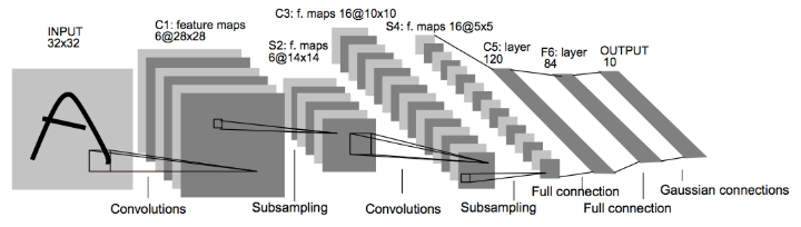
上面是LeNet神经网络结构
37.1 Load Data
Load the MNIST data, which comes pre-loaded with TensorFlow.
from tensorflow.examples.tutorials.mnist import input_data

mnist = input_data.read_data_sets("MNIST_data/", reshape=False)
X_train, y_train           = mnist.train.images, mnist.train.labels
X_validation, y_validation = mnist.validation.images, mnist.validation.labels
X_test, y_test             = mnist.test.images, mnist.test.labels

assert(len(X_train) == len(y_train))
assert(len(X_validation) == len(y_validation))
assert(len(X_test) == len(y_test))

print()
print("Image Shape: {}".format(X_train[0].shape))
print()
print("Training Set:   {} samples".format(len(X_train)))
print("Validation Set: {} samples".format(len(X_validation)))
print("Test Set:       {} samples".format(len(X_test)))
Extracting MNIST_data/train-images-idx3-ubyte.gz
Extracting MNIST_data/train-labels-idx1-ubyte.gz
Extracting MNIST_data/t10k-images-idx3-ubyte.gz
Extracting MNIST_data/t10k-labels-idx1-ubyte.gz

Image Shape: (28, 28, 1)

Training Set:   55000 samples
Validation Set: 5000 samples
Test Set:       10000 samples
The MNIST data that TensorFlow pre-loads comes as 28x28x1 images.
However, the LeNet architecture only accepts 32x32xC images, where C is the number of color channels.
In order to reformat the MNIST data into a shape that LeNet will accept, we pad the data with two rows of zeros on the top and bottom, and two columns of zeros on the left and right (28+2+2 = 32).
import numpy as np

# Pad images with 0s
X_train      = np.pad(X_train, ((0,0),(2,2),(2,2),(0,0)), 'constant')
X_validation = np.pad(X_validation, ((0,0),(2,2),(2,2),(0,0)), 'constant')
X_test       = np.pad(X_test, ((0,0),(2,2),(2,2),(0,0)), 'constant')

print("Updated Image Shape: {}".format(X_train[0].shape))
Updated Image Shape: (32, 32, 1)
pad函数的用法,参考numpy.pad
37.2 Visualize Data
import random
import numpy as np
import matplotlib.pyplot as plt
%matplotlib inline

index = random.randint(0, len(X_train))
image = X_train[index].squeeze()

plt.figure(figsize=(1,1))
plt.imshow(image, cmap="gray")
print(y_train[index])

37.3 Preprocess Data
将数据随机打乱。
from sklearn.utils import shuffle

X_train, y_train = shuffle(X_train, y_train)
37.4 Setup TensorFlow
The `EPOCH` and `BATCH_SIZE` values affect the training speed and model accuracy.
import tensorflow as tf

EPOCHS = 10
BATCH_SIZE = 128
37.4 TODO: Implement LeNet-5
Implement the LeNet-5 neural network architecture.
This is the only cell you need to edit.
Input
The LeNet architecture accepts a 32x32xC image as input, where C is the number of color channels. Since MNIST images are grayscale, C is 1 in this case.
Architecture
Layer 1: Convolutional. The output shape should be 28x28x6.
Activation. Your choice of activation function.
Pooling. The output shape should be 14x14x6.
Layer 2: Convolutional. The output shape should be 10x10x16.
Activation. Your choice of activation function.
Pooling. The output shape should be 5x5x16.
Flatten. Flatten the output shape of the final pooling layer such that it’s 1D instead of 3D. The easiest way to do is by using tf.contrib.layers.flatten, which is already imported for you.
Layer 3: Fully Connected. This should have 120 outputs.
Activation. Your choice of activation function.
Layer 4: Fully Connected. This should have 84 outputs.
Activation. Your choice of activation function.
Layer 5: Fully Connected (Logits). This should have 10 outputs.
Output
Return the result of the 2nd fully connected layer.
代码
from tensorflow.contrib.layers import flatten

def LeNet(x):
    # Arguments used for tf.truncated_normal, randomly defines variables for the weights and biases for each layer
    mu = 0
    sigma = 0.1

    # TODO: Layer 1: Convolutional. Input = 32x32x1. Output = 28x28x6.
    filter_weights = tf.Variable(tf.truncated_normal((5, 5, 1, 6), mean = mu, stddev = sigma)) # (height, width, input_depth, output_depth)
    filter_bias = tf.Variable(tf.zeros(6))
    strides = [1, 1, 1, 1] # (batch, height, width, depth)
    padding = 'VALID'
    conv_1 = tf.nn.conv2d(x, filter_weights, strides, padding) + filter_bias

    # TODO: Activation.
    conv_1 = tf.nn.relu(conv_1)

    # TODO: Pooling. Input = 28x28x6. Output = 14x14x6.
    conv_1 = tf.nn.max_pool(conv_1, ksize=[1, 2, 2, 1], strides=[1, 2, 2, 1], padding='VALID')

    # TODO: Layer 2: Convolutional. Output = 10x10x16.
    filter_weights = tf.Variable(tf.truncated_normal((5, 5, 6, 16), mean = mu, stddev = sigma)) # (height, width, input_depth, output_depth)
    filter_bias = tf.Variable(tf.zeros(16))
    strides = [1, 1, 1, 1] # (batch, height, width, depth)
    padding = 'VALID'
    conv_2 = tf.nn.conv2d(conv_1, filter_weights, strides, padding) + filter_bias

    # TODO: Activation.
    conv_2 = tf.nn.relu(conv_2)

    # TODO: Pooling. Input = 10x10x16. Output = 5x5x16.
    conv_2 = tf.nn.max_pool(conv_2, ksize=[1, 2, 2, 1], strides=[1, 2, 2, 1], padding='VALID')

    # TODO: Flatten. Input = 5x5x16. Output = 400.
    fc0 = flatten(conv_2)

    # TODO: Layer 3: Fully Connected. Input = 400. Output = 120.
    wd1 = tf.Variable(tf.truncated_normal(shape=(400, 120), mean = mu, stddev = sigma))
    bd1 = tf.Variable(tf.zeros(120))
    fc1 = tf.add(tf.matmul(fc0,wd1), bd1)

    # TODO: Activation.
    fc1 = tf.nn.relu(fc1)

    # TODO: Layer 4: Fully Connected. Input = 120. Output = 84.
    wd2 = tf.Variable(tf.truncated_normal(shape=(120, 84), mean = mu, stddev = sigma))
    bd2 = tf.Variable(tf.zeros(84))
    fc2 = tf.add(tf.matmul(fc1, wd2), bd2)

    # TODO: Activation.
    fc2 = tf.nn.relu(fc2)

    # TODO: Layer 5: Fully Connected. Input = 84. Output = 10.

    wd3 = tf.Variable(tf.truncated_normal(shape=(84, 10), mean = mu, stddev = sigma))
    bd3 = tf.Variable(tf.zeros(10))
    logits = tf.add(tf.matmul(fc2, wd3), bd3)

    return logits
37.5 Features and Labels
Train LeNet to classify MNIST data.
xis a placeholder for a batch of input images.yis a placeholder for a batch of output labels.
x = tf.placeholder(tf.float32, (None, 32, 32, 1))
y = tf.placeholder(tf.int32, (None))
one_hot_y = tf.one_hot(y, 10)
37.6 Training Pipeline
Create a training pipeline that uses the model to classify MNIST data.
rate = 0.001

logits = LeNet(x)
cross_entropy = tf.nn.softmax_cross_entropy_with_logits(labels=one_hot_y, logits=logits)
loss_operation = tf.reduce_mean(cross_entropy)
optimizer = tf.train.AdamOptimizer(learning_rate = rate)
training_operation = optimizer.minimize(loss_operation)
37.7 Model Evaluation
Evaluate how well the loss and accuracy of the model for a given dataset.
correct_prediction = tf.equal(tf.argmax(logits, 1), tf.argmax(one_hot_y, 1))
accuracy_operation = tf.reduce_mean(tf.cast(correct_prediction, tf.float32))
saver = tf.train.Saver()

def evaluate(X_data, y_data):
    num_examples = len(X_data)
    total_accuracy = 0
    sess = tf.get_default_session()
    for offset in range(0, num_examples, BATCH_SIZE):
        batch_x, batch_y = X_data[offset:offset+BATCH_SIZE], y_data[offset:offset+BATCH_SIZE]
        accuracy = sess.run(accuracy_operation, feed_dict={x: batch_x, y: batch_y})
        total_accuracy += (accuracy * len(batch_x))
    return total_accuracy / num_examples
37.8 Train the Model
Run the training data through the training pipeline to train the model.
Before each epoch, shuffle the training set.
After each epoch, measure the loss and accuracy of the validation set.
Save the model after training.
with tf.Session() as sess:
    sess.run(tf.global_variables_initializer())
    num_examples = len(X_train)

    print("Training...")
    print()
    for i in range(EPOCHS):
        X_train, y_train = shuffle(X_train, y_train)
        for offset in range(0, num_examples, BATCH_SIZE):
            end = offset + BATCH_SIZE
            batch_x, batch_y = X_train[offset:end], y_train[offset:end]
            sess.run(training_operation, feed_dict={x: batch_x, y: batch_y})

        validation_accuracy = evaluate(X_validation, y_validation)
        print("EPOCH {} ...".format(i+1))
        print("Validation Accuracy = {:.3f}".format(validation_accuracy))
        print()

    saver.save(sess, './lenet')
    print("Model saved")
输出:
Training...

EPOCH 1 ...
Validation Accuracy = 0.969

...

EPOCH 10 ...
Validation Accuracy = 0.988

Model saved
37.9 Evaluate the Model
Once you are completely satisfied with your model, evaluate the performance of the model on the test set.
Be sure to only do this once!
If you were to measure the performance of your trained model on the test set, then improve your model, and then measure the performance of your model on the test set again, that would invalidate your test results. You wouldn’t get a true measure of how well your model would perform against real data.
with tf.Session() as sess:
    saver.restore(sess, tf.train.latest_checkpoint('.'))

    test_accuracy = evaluate(X_test, y_test)
    print("Test Accuracy = {:.3f}".format(test_accuracy))
最终输出:
INFO:tensorflow:Restoring parameters from ./lenet
Test Accuracy = 0.989
37. Lab代码解析
代码整体结构如下:

37.1 LeNet的udacity代码:
from tensorflow.contrib.layers import flatten

def LeNet(x):
    # Arguments used for tf.truncated_normal, randomly defines variables for the weights and biases for each layer
    mu = 0
    sigma = 0.1

    # SOLUTION: Layer 1: Convolutional. Input = 32x32x1. Output = 28x28x6.
    conv1_W = tf.Variable(tf.truncated_normal(shape=(5, 5, 1, 6), mean = mu, stddev = sigma))
    conv1_b = tf.Variable(tf.zeros(6))
    conv1   = tf.nn.conv2d(x, conv1_W, strides=[1, 1, 1, 1], padding='VALID') + conv1_b

    # SOLUTION: Activation.
    conv1 = tf.nn.relu(conv1)

    # SOLUTION: Pooling. Input = 28x28x6. Output = 14x14x6.
    conv1 = tf.nn.max_pool(conv1, ksize=[1, 2, 2, 1], strides=[1, 2, 2, 1], padding='VALID')

    # SOLUTION: Layer 2: Convolutional. Output = 10x10x16.
    conv2_W = tf.Variable(tf.truncated_normal(shape=(5, 5, 6, 16), mean = mu, stddev = sigma))
    conv2_b = tf.Variable(tf.zeros(16))
    conv2   = tf.nn.conv2d(conv1, conv2_W, strides=[1, 1, 1, 1], padding='VALID') + conv2_b

    # SOLUTION: Activation.
    conv2 = tf.nn.relu(conv2)

    # SOLUTION: Pooling. Input = 10x10x16. Output = 5x5x16.
    conv2 = tf.nn.max_pool(conv2, ksize=[1, 2, 2, 1], strides=[1, 2, 2, 1], padding='VALID')

    # SOLUTION: Flatten. Input = 5x5x16. Output = 400.
    fc0   = flatten(conv2)

    # SOLUTION: Layer 3: Fully Connected. Input = 400. Output = 120.
    fc1_W = tf.Variable(tf.truncated_normal(shape=(400, 120), mean = mu, stddev = sigma))
    fc1_b = tf.Variable(tf.zeros(120))
    fc1   = tf.matmul(fc0, fc1_W) + fc1_b

    # SOLUTION: Activation.
    fc1    = tf.nn.relu(fc1)

    # SOLUTION: Layer 4: Fully Connected. Input = 120. Output = 84.
    fc2_W  = tf.Variable(tf.truncated_normal(shape=(120, 84), mean = mu, stddev = sigma))
    fc2_b  = tf.Variable(tf.zeros(84))
    fc2    = tf.matmul(fc1, fc2_W) + fc2_b

    # SOLUTION: Activation.
    fc2    = tf.nn.relu(fc2)

    # SOLUTION: Layer 5: Fully Connected. Input = 84. Output = 10.
    fc3_W  = tf.Variable(tf.truncated_normal(shape=(84, 10), mean = mu, stddev = sigma))
    fc3_b  = tf.Variable(tf.zeros(10))
    logits = tf.matmul(fc2, fc3_W) + fc3_b

    return logits
- Layer1中,ouput的depth为6,说明滤波器的depth为6,偏置为6,另外,input为32×32,output为28×28,说明stride只能为1,计算可知道滤波器的长宽为(32-28+1)/1 = 5。
- Layer1中,池化前后分别为28×28和14×14,说明池化是以2×2为单位,且步长为2,示例图如下:

- Layer2也是一样方法
- Layer3,通过全连接层的计算法,即直接用权重乘以input,加上偏置,得到Layer3的结果,再通过激活层进行处理
- Layer4和Layer5与Layer3相同的方法
38. CNNs - Additional Resources
Additional Resources: There are many wonderful free resources that allow you to go into more depth around Convolutional Neural Networks. In this course, our goal is to give you just enough intuition to start applying this concept on real world problems so you have enough of an exposure to explore more on your own. We strongly encourage you to explore some of these resources more to reinforce your intuition and explore different ideas.
These are the resources we recommend in particular:
- Andrej Karpathy’s CS231n Stanford course on Convolutional Neural Networks.
- Michael Nielsen’s free book on Deep Learning.
- Goodfellow, Bengio, and Courville’s more advanced free book on Deep Learning.