- 1. LeNet神经网络结构
- 2. Load Data
- 3. Visualize Data
- 4. Preprocess Data
- 5. Setup TensorFlow
- 6. TODO: Implement LeNet-5
- 7. Features and Labels
- 8. Training Pipeline
- 9. Model Evaluation
- 10. Train the Model
- 11. Evaluate the Model
这一章是针对上一章最后一个Lab的讲解。
代码整体结构如下:

- Layer1中,ouput的depth为6,说明滤波器的depth为6,偏置为6,另外,input为32×32,output为28×28,说明stride只能为1,计算可知道滤波器的长宽为(32-28+1)/1 = 5。
- Layer1中,池化前后分别为28×28和14×14,说明池化是以2×2为单位,且步长为2,示例图如下:

- Layer2也是一样方法
- Layer3,通过全连接层的计算法,即直接用权重乘以input,加上偏置,得到Layer3的结果,再通过激活层进行处理
- Layer4和Layer5与Layer3相同的方法
1. LeNet神经网络结构
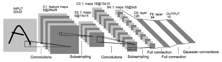
- 输入数据是32*32的图像。
- 经过卷积层C1,再经过二次抽样层(这里是池化层)S2。
- 再经过卷积层C3,池化层S4。
- 最后最末端有三个完全连接的全连接层,其中包括最后的输出层。
2. Load Data
Load the MNIST data, which comes pre-loaded with TensorFlow.
读取数据,并分为训练集/验证集/测试集
from tensorflow.examples.tutorials.mnist import input_data

mnist = input_data.read_data_sets("MNIST_data/", reshape=False)
X_train, y_train           = mnist.train.images, mnist.train.labels
X_validation, y_validation = mnist.validation.images, mnist.validation.labels
X_test, y_test             = mnist.test.images, mnist.test.labels

assert(len(X_train) == len(y_train))
assert(len(X_validation) == len(y_validation))
assert(len(X_test) == len(y_test))

print()
print("Image Shape: {}".format(X_train[0].shape))
print()
print("Training Set:   {} samples".format(len(X_train)))
print("Validation Set: {} samples".format(len(X_validation)))
print("Test Set:       {} samples".format(len(X_test)))
Extracting MNIST_data/train-images-idx3-ubyte.gz
Extracting MNIST_data/train-labels-idx1-ubyte.gz
Extracting MNIST_data/t10k-images-idx3-ubyte.gz
Extracting MNIST_data/t10k-labels-idx1-ubyte.gz

Image Shape: (28, 28, 1)

Training Set:   55000 samples
Validation Set: 5000 samples
Test Set:       10000 samples
The MNIST data that TensorFlow pre-loads comes as 28x28x1 images.
However, the LeNet architecture only accepts 32x32xC images, where C is the number of color channels.
In order to reformat the MNIST data into a shape that LeNet will accept, we pad the data with two rows of zeros on the top and bottom, and two columns of zeros on the left and right (28+2+2 = 32).
import numpy as np

# Pad images with 0s
X_train      = np.pad(X_train, ((0,0),(2,2),(2,2),(0,0)), 'constant')
X_validation = np.pad(X_validation, ((0,0),(2,2),(2,2),(0,0)), 'constant')
X_test       = np.pad(X_test, ((0,0),(2,2),(2,2),(0,0)), 'constant')

print("Updated Image Shape: {}".format(X_train[0].shape))
Updated Image Shape: (32, 32, 1)
pad函数的用法,参考numpy.pad
3. Visualize Data
随机选取一张图片,并可视化:
import random
import numpy as np
import matplotlib.pyplot as plt
%matplotlib inline

index = random.randint(0, len(X_train))
image = X_train[index].squeeze()

plt.figure(figsize=(1,1))
plt.imshow(image, cmap="gray")
print(y_train[index])

4. Preprocess Data
打乱训练数据集的顺序十分必要,否则数据的顺序可能会对网络的性能产生影响:
from sklearn.utils import shuffle

X_train, y_train = shuffle(X_train, y_train)
5. Setup TensorFlow
- epochs:告诉TensorFlow需要在神经网络中运行多少次训练数据,一般来说,epoch越大精度越高,但耗时也越长
- batch_size:告诉TensorFlow每次在神经网络中运行的训练图像有多少个,批量越大,训练速度越快,但是所使用的内存也越大
The `EPOCH` and `BATCH_SIZE` values affect the training speed and model accuracy.
import tensorflow as tf

EPOCHS = 10
BATCH_SIZE = 128
6. TODO: Implement LeNet-5
Implement the LeNet-5 neural network architecture.
This is the only cell you need to edit.
Input
The LeNet architecture accepts a 32x32xC image as input, where C is the number of color channels. Since MNIST images are grayscale, C is 1 in this case.
Architecture
Layer 1: Convolutional. The output shape should be 28x28x6.
Activation. Your choice of activation function.
Pooling. The output shape should be 14x14x6.
Layer 2: Convolutional. The output shape should be 10x10x16.
Activation. Your choice of activation function.
Pooling. The output shape should be 5x5x16.
Flatten. Flatten the output shape of the final pooling layer such that it’s 1D instead of 3D. The easiest way to do is by using tf.contrib.layers.flatten, which is already imported for you.
Layer 3: Fully Connected. This should have 120 outputs.
Activation. Your choice of activation function.
Layer 4: Fully Connected. This should have 84 outputs.
Activation. Your choice of activation function.
Layer 5: Fully Connected (Logits). This should have 10 outputs.
Output
Return the result of the 2nd fully connected layer.
代码
- 设定mu和sigma超参数
- 再定义各个layer的权重和偏置,并用权重和偏置生成对应的layer
- 最后的output layer是10个数,即数字(0-9)的识别结果。
from tensorflow.contrib.layers import flatten

def LeNet(x):
    # Arguments used for tf.truncated_normal, randomly defines variables for the weights and biases for each layer
    mu = 0
    sigma = 0.1

    # SOLUTION: Layer 1: Convolutional. Input = 32x32x1. Output = 28x28x6.
    conv1_W = tf.Variable(tf.truncated_normal(shape=(5, 5, 1, 6), mean = mu, stddev = sigma))
    conv1_b = tf.Variable(tf.zeros(6))
    conv1   = tf.nn.conv2d(x, conv1_W, strides=[1, 1, 1, 1], padding='VALID') + conv1_b

    # SOLUTION: Activation.
    conv1 = tf.nn.relu(conv1)

    # SOLUTION: Pooling. Input = 28x28x6. Output = 14x14x6.
    conv1 = tf.nn.max_pool(conv1, ksize=[1, 2, 2, 1], strides=[1, 2, 2, 1], padding='VALID')

    # SOLUTION: Layer 2: Convolutional. Output = 10x10x16.
    conv2_W = tf.Variable(tf.truncated_normal(shape=(5, 5, 6, 16), mean = mu, stddev = sigma))
    conv2_b = tf.Variable(tf.zeros(16))
    conv2   = tf.nn.conv2d(conv1, conv2_W, strides=[1, 1, 1, 1], padding='VALID') + conv2_b

    # SOLUTION: Activation.
    conv2 = tf.nn.relu(conv2)

    # SOLUTION: Pooling. Input = 10x10x16. Output = 5x5x16.
    conv2 = tf.nn.max_pool(conv2, ksize=[1, 2, 2, 1], strides=[1, 2, 2, 1], padding='VALID')

    # SOLUTION: Flatten. Input = 5x5x16. Output = 400.
    fc0   = flatten(conv2)

    # SOLUTION: Layer 3: Fully Connected. Input = 400. Output = 120.
    fc1_W = tf.Variable(tf.truncated_normal(shape=(400, 120), mean = mu, stddev = sigma))
    fc1_b = tf.Variable(tf.zeros(120))
    fc1   = tf.matmul(fc0, fc1_W) + fc1_b

    # SOLUTION: Activation.
    fc1    = tf.nn.relu(fc1)

    # SOLUTION: Layer 4: Fully Connected. Input = 120. Output = 84.
    fc2_W  = tf.Variable(tf.truncated_normal(shape=(120, 84), mean = mu, stddev = sigma))
    fc2_b  = tf.Variable(tf.zeros(84))
    fc2    = tf.matmul(fc1, fc2_W) + fc2_b

    # SOLUTION: Activation.
    fc2    = tf.nn.relu(fc2)

    # SOLUTION: Layer 5: Fully Connected. Input = 84. Output = 10.
    fc3_W  = tf.Variable(tf.truncated_normal(shape=(84, 10), mean = mu, stddev = sigma))
    fc3_b  = tf.Variable(tf.zeros(10))
    logits = tf.matmul(fc2, fc3_W) + fc3_b

    return logits
7. Features and Labels
Train LeNet to classify MNIST data.
xis a placeholder for a batch of input images.yis a placeholder for a batch of output labels.
x = tf.placeholder(tf.float32, (None, 32, 32, 1))
y = tf.placeholder(tf.int32, (None))
one_hot_y = tf.one_hot(y, 10)
8. Training Pipeline
Create a training pipeline that uses the model to classify MNIST data.
- rate决定了TensorFlow更新神经网络中权重的速度。
softmax_cross_entropy_with_logits,计算预测结果与标签之间的交叉熵。reduce_mean,求出所有训练图像的交叉熵平均值。AdamOptimizer,使用Adam算法来最小化损失函数,是优化后的随机梯度下降算法。- 最后,在优化器上运行最小化函数,通过反向传播,以最小化训练期间的损失函数值,更新神经网络。
rate = 0.001

logits = LeNet(x)
cross_entropy = tf.nn.softmax_cross_entropy_with_logits(labels=one_hot_y, logits=logits)
loss_operation = tf.reduce_mean(cross_entropy)
optimizer = tf.train.AdamOptimizer(learning_rate = rate)
training_operation = optimizer.minimize(loss_operation)
9. Model Evaluation
Evaluate how well the loss and accuracy of the model for a given dataset.
这次的目的是评估模型,这里创建管道来评估模型性能:
- 第一步,计算出模型预测的对数几率,然后与热编码后的标签进行比对,再判断模型给出的预测是否正确。
- 第二步,计算模型的整体准确度,模型的整体准确度是所有预测的准确度的平均值
这两步构成整个评估管道。
evaluate()函数,输入一个数据集,设定一些初始变量,然后分批处理数据集,并在整个评估管道中运行数据集。该函数计算出每批次的准确度
correct_prediction = tf.equal(tf.argmax(logits, 1), tf.argmax(one_hot_y, 1))
accuracy_operation = tf.reduce_mean(tf.cast(correct_prediction, tf.float32))
saver = tf.train.Saver()

def evaluate(X_data, y_data):
    num_examples = len(X_data)
    total_accuracy = 0
    sess = tf.get_default_session()
    for offset in range(0, num_examples, BATCH_SIZE):
        batch_x, batch_y = X_data[offset:offset+BATCH_SIZE], y_data[offset:offset+BATCH_SIZE]
        accuracy = sess.run(accuracy_operation, feed_dict={x: batch_x, y: batch_y})
        total_accuracy += (accuracy * len(batch_x))
    return total_accuracy / num_examples
10. Train the Model
Run the training data through the training pipeline to train the model. Before each epoch, shuffle the training set. After each epoch, measure the loss and accuracy of the validation set. Save the model after training.
- 创建TensorFlow会话并初始化变量。
- 根据epochs决定数据训练的轮数。
- 然后根据BATCH_SIZE分成几批数据,分批训练模型。
- 每轮Epoch结束后,利用交叉验证集评估模型。
- 最后保存到文件。
with tf.Session() as sess:
    sess.run(tf.global_variables_initializer())
    num_examples = len(X_train)

    print("Training...")
    print()
    for i in range(EPOCHS):
        X_train, y_train = shuffle(X_train, y_train)
        for offset in range(0, num_examples, BATCH_SIZE):
            end = offset + BATCH_SIZE
            batch_x, batch_y = X_train[offset:end], y_train[offset:end]
            sess.run(training_operation, feed_dict={x: batch_x, y: batch_y})

        validation_accuracy = evaluate(X_validation, y_validation)
        print("EPOCH {} ...".format(i+1))
        print("Validation Accuracy = {:.3f}".format(validation_accuracy))
        print()

    saver.save(sess, './lenet')
    print("Model saved")
输出:
Training...

EPOCH 1 ...
Validation Accuracy = 0.969

...

EPOCH 10 ...
Validation Accuracy = 0.988

Model saved
11. Evaluate the Model
Once you are completely satisfied with your model, evaluate the performance of the model on the test set.
Be sure to only do this once!
If you were to measure the performance of your trained model on the test set, then improve your model, and then measure the performance of your model on the test set again, that would invalidate your test results. You wouldn’t get a true measure of how well your model would perform against real data.
with tf.Session() as sess:
    saver.restore(sess, tf.train.latest_checkpoint('.'))

    test_accuracy = evaluate(X_test, y_test)
    print("Test Accuracy = {:.3f}".format(test_accuracy))
最终输出:
INFO:tensorflow:Restoring parameters from ./lenet
Test Accuracy = 0.989