- 0. LeNet for Traffic Signs
- 1. Load The Data
- 2. Dataset Summary & Exploration
- 3. Design and Test a Model Architecture
- 4. Test a Model on New Images
- 5. 小结
这个project中需要构建一个深度神经网络,对交通标志进行分类,比如是停止或是前行标志。
下面内容是Lesson15中的第9和10,讲解了如何通过LeNet来完成这个project。
0. LeNet for Traffic Signs
0.1 LeNet for Traffic Signs
可以使用上一章的神经网络去训练交通信号灯识别:
- Reset the kernel and clear the output to ensure you have a fresh start.
- Clear the cells that load the MNIST data and replace it with code to load the traffic sign data.(the code is in the notebook for the traffic sign classifier project)
- The traffic sign data does not come with a validation set, you can use the train test split function in the SKLearn library though to slice off a validation set from the training set.
You can proceed to pre-process the data and set up TensorFlow just as we dit for MNIST., but you’ll have to make a few changes to the LeNet architecture though.
- The traffic sign images are in color not gray scale, so the input depth should be three to match the three RGB color channels.
- At the ouput layer the traffic sign classifier has 43 classes, whereas MNIST only had 10 so you’ll have to change that.
- When you set up the TensorFlow placeholders, you’ll have to update the input and output shapes again to match the shapes of the new dataset.
通过上述的改造,就可以大致使用该神经网络去训练信号灯数据了,下面是进一步的改进方法:
- experiment with different network architectures, or just change the dimensions of the LeNet layers
- add regularization features like drop out or L2 regularization to make sure the network doesn’t overfit the training data
- tune the hyperparameters
- improve the data pre-processing with steps like normalization and setting a zero mean
- augment the training data by rotating or shifting images or by changing colors
0.2 Visualizing Layers
神经网络对于我们训练来说类似一个黑盒,通过一些技巧将各个层的信息可视化,可以看出神经网络究竟对什么样的信息感兴趣。
下面的这个函数,能将TensorFlow中指定的权重层可视化:
- 输入数据1:图片数据,可以是训练中的数据,也可以是提供的input
- 输入数据2:the Tensorflow variable name that represents the layer’s state during the training process
如果是想确认LeNet中第二层卷积层的特征图,输入数据则是conv2 **和tf_activation **。
示例代码如下:
# image_input: the test image being fed into the network to produce the feature maps
# tf_activation: should be a tf variable name used during your training procedure that represents the calculated state of a specific weight layer
# Note: that to get access to tf_activation, the session should be interactive which can be achieved with the following commands.
# sess = tf.InteractiveSession()
# sess.as_default()

# activation_min/max: can be used to view the activation contrast in more detail, by default matplot sets min and max to the actual min and    max values of the output
# plt_num: used to plot out multiple different weight feature map sets on the same block, just extend the plt number for each new feature map entry

def outputFeatureMap(image_input, tf_activation, activation_min=-1, activation_max=-1 ,plt_num=1):
    # Here make sure to preprocess your image_input in a way your network expects
    # with size, normalization, ect if needed
    # image_input =
    # Note: x should be the same name as your network's tensorflow data placeholder variable
    # If you get an error tf_activation is not defined it maybe having trouble accessing the variable from inside a function
    activation = tf_activation.eval(session=sess,feed_dict={x : image_input})
    featuremaps = activation.shape[3]
    plt.figure(plt_num, figsize=(15,15))
    for featuremap in range(featuremaps):
        plt.subplot(6,8, featuremap+1) # sets the number of feature maps to show on each row and column
        plt.title('FeatureMap ' + str(featuremap)) # displays the feature map number
        if activation_min != -1 & activation_max != -1:
            plt.imshow(activation[0,:,:, featuremap], interpolation="nearest", vmin =activation_min, vmax=activation_max, cmap="gray")
        elif activation_max != -1:
            plt.imshow(activation[0,:,:, featuremap], interpolation="nearest", vmax=activation_max, cmap="gray")
        elif activation_min !=-1:
            plt.imshow(activation[0,:,:, featuremap], interpolation="nearest", vmin=activation_min, cmap="gray")
        else:
            plt.imshow(activation[0,:,:, featuremap], interpolation="nearest", cmap="gray")
1. Load The Data
# Load pickled data
import pickle
import numpy as np

# TODO: Fill this in based on where you saved the training and testing data

training_file = "../data/train.p"
validation_file= "../data/valid.p"
testing_file = "../data/test.p"

with open(training_file, mode='rb') as f:
    train = pickle.load(f)
with open(validation_file, mode='rb') as f:
    valid = pickle.load(f)
with open(testing_file, mode='rb') as f:
    test = pickle.load(f)

X_train, y_train = train['features'], train['labels']
X_valid, y_valid = valid['features'], valid['labels']
X_test, y_test = test['features'], test['labels']
2. Dataset Summary & Exploration
上面pickled数据类型是字典:
'features'信号灯图片像素数据的4维数组,包含(Number,width,height,channels).'labels'信号灯图片的标签数据.signnames.csv中有每个label对应的实际信号灯意义数据.'sizes'包含元组的list, (width, height) representing the original width and height the image.'coords'包含元组的list, (x1, y1, x2, y2) representing coordinates of a bounding box around the sign in the image.
2.1 Data summary
### Replace each question mark with the appropriate value.
### Use python, pandas or numpy methods rather than hard coding the results

# TODO: Number of training examples
n_train = len(X_train)

# TODO: Number of validation examples
n_validation = len(X_valid)

# TODO: Number of testing examples.
n_test = len(X_test)

# TODO: What's the shape of an traffic sign image?
image_shape = X_train[0].shape

# TODO: How many unique classes/labels there are in the dataset.
n_classes = len(np.unique(y_train))

print("Number of training examples =", n_train)
print("Number of validation examples =", n_validation)
print("Number of testing examples =", n_test)
print("Image data shape =", image_shape)
print("Number of classes =", n_classes)
Number of training examples = 34799
Number of validation examples = 4410
Number of testing examples = 12630
Image data shape = (32, 32, 3)
Number of classes = 43
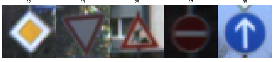
2.2 Include an exploratory visualization of the dataset
### Data exploration visualization code goes here.
### Feel free to use as many code cells as needed.
import matplotlib.pyplot as plt
# Visualizations will be shown in the notebook.
%matplotlib inline
import random

fig, axs = plt.subplots(1,5, figsize=(15, 6))
fig.subplots_adjust(hspace = .2, wspace=.001)
axs = axs.ravel()
for i in range(5):
    index = random.randint(0, len(X_train))
    image = X_train[index]
    axs[i].axis('off')
    axs[i].imshow(image)
    axs[i].set_title(y_train[index])
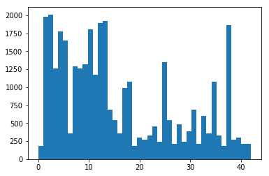
plt.hist(y_train, bins = n_classes)
(array([  180.,  1980.,  2010.,  1260.,  1770.,  1650.,   360.,  1290.,
         1260.,  1320.,  1800.,  1170.,  1890.,  1920.,   690.,   540.,
          360.,   990.,  1080.,   180.,   300.,   270.,   330.,   450.,
          240.,  1350.,   540.,   210.,   480.,   240.,   390.,   690.,
          210.,   599.,   360.,  1080.,   330.,   180.,  1860.,   270.,
          300.,   210.,   210.]),
 array([  0.        ,   0.97674419,   1.95348837,   2.93023256,
          3.90697674,   4.88372093,   5.86046512,   6.8372093 ,
          7.81395349,   8.79069767,   9.76744186,  10.74418605,
         11.72093023,  12.69767442,  13.6744186 ,  14.65116279,
         15.62790698,  16.60465116,  17.58139535,  18.55813953,
         19.53488372,  20.51162791,  21.48837209,  22.46511628,
         23.44186047,  24.41860465,  25.39534884,  26.37209302,
         27.34883721,  28.3255814 ,  29.30232558,  30.27906977,
         31.25581395,  32.23255814,  33.20930233,  34.18604651,
         35.1627907 ,  36.13953488,  37.11627907,  38.09302326,
         39.06976744,  40.04651163,  41.02325581,  42.        ]),
 <a list of 43 Patch objects>)
3. Design and Test a Model Architecture
3.1 Pre-process the Data Set
- 将数据打乱
- 将数据正规化到[-1,1]
- 将label数据进行one-hot编码
### Preprocess the data here. It is required to normalize the data. Other preprocessing steps could include
import cv2
from sklearn.utils import shuffle

X_train, y_train = shuffle(X_train, y_train)
X_valid, y_valid = shuffle(X_valid, y_valid)
X_test, y_test = shuffle(X_test, y_test)
from sklearn.model_selection import train_test_split
from sklearn import preprocessing

def normalize(data):
    return (data.astype('float32') -128) / 128

def label_binarizer(labels):
    lb = preprocessing.LabelBinarizer()
    lb.fit(labels)
    return lb

def preprocess(X_train, y_train, X_valid, y_valid, X_test, y_test):
    X_train = normalize(X_train)
    X_valid = normalize(X_valid)
    X_test = normalize(X_test)

    # One hot encode labels
    lb = label_binarizer(y_train)

    y_train = lb.transform(y_train)
    y_valid = lb.transform(y_valid)
    y_test = lb.transform(y_test)

    return X_train, y_train, X_valid, y_valid, X_test, y_test

X_train, y_train, X_valid, y_valid, X_test, y_test = preprocess(X_train, y_train, X_valid, y_valid, X_test, y_test)
3.2 Model Architecture
基于LeNet改造网络,添加了新的Drop层,另外根据input数据修改了shape等参数。模型结构如下:
| Layer | Description |
|---|---|
| Input | 32x32x3 RGB image |
| Convolution 5x5 | 2x2 stride, valid padding, outputs 28x28x6 |
| RELU | |
| Max pooling | 2x2 stride, outputs 14x14x6 |
| Convolution 5x5 | 2x2 stride, valid padding, outputs 10x10x16 |
| RELU | |
| Max pooling | 2x2 stride, outputs 5x5x6 |
| Fully connected | input 400, output 120 |
| RELU | |
| Dropout | 50% keep |
| Fully connected | input 120, output 84 |
| RELU | |
| Dropout | 50% keep |
| Fully connected | input 84, output 43 |
import tensorflow as tf
from tensorflow.contrib.layers import flatten

def LeNet(x):
    # Arguments used for tf.truncated_normal, randomly defines variables for the weights and biases for each layer
    mu = 0
    sigma = 0.1

    # SOLUTION: Layer 1: Convolutional. Input = 32x32x3. Output = 28x28x6.
    conv1_W = tf.Variable(tf.truncated_normal(shape=(5, 5, 3, 6), mean = mu, stddev = sigma))
    conv1_b = tf.Variable(tf.zeros(6))
    conv1   = tf.nn.conv2d(x, conv1_W, strides=[1, 1, 1, 1], padding='VALID') + conv1_b

    # SOLUTION: Activation.
    conv1 = tf.nn.relu(conv1)

    # SOLUTION: Pooling. Input = 28x28x6. Output = 14x14x6.
    conv1 = tf.nn.max_pool(conv1, ksize=[1, 2, 2, 1], strides=[1, 2, 2, 1], padding='VALID')

    # SOLUTION: Layer 2: Convolutional. Output = 10x10x16.
    conv2_W = tf.Variable(tf.truncated_normal(shape=(5, 5, 6, 16), mean = mu, stddev = sigma))
    conv2_b = tf.Variable(tf.zeros(16))
    conv2   = tf.nn.conv2d(conv1, conv2_W, strides=[1, 1, 1, 1], padding='VALID') + conv2_b

    # SOLUTION: Activation.
    conv2 = tf.nn.relu(conv2)

    # SOLUTION: Pooling. Input = 10x10x16. Output = 5x5x16.
    conv2 = tf.nn.max_pool(conv2, ksize=[1, 2, 2, 1], strides=[1, 2, 2, 1], padding='VALID')

    # SOLUTION: Flatten. Input = 5x5x16. Output = 400.
    fc0   = flatten(conv2)

    # SOLUTION: Layer 3: Fully Connected. Input = 400. Output = 120.
    fc1_W = tf.Variable(tf.truncated_normal(shape=(400, 120), mean = mu, stddev = sigma))
    fc1_b = tf.Variable(tf.zeros(120))
    fc1   = tf.matmul(fc0, fc1_W) + fc1_b

    # SOLUTION: Activation.
    fc1    = tf.nn.relu(fc1)
    fc1 = tf.nn.dropout(fc1, keep_prob)

    # SOLUTION: Layer 4: Fully Connected. Input = 120. Output = 84.
    fc2_W  = tf.Variable(tf.truncated_normal(shape=(120, 84), mean = mu, stddev = sigma))
    fc2_b  = tf.Variable(tf.zeros(84))
    fc2    = tf.matmul(fc1, fc2_W) + fc2_b

    # SOLUTION: Activation.
    fc2    = tf.nn.relu(fc2)
    fc2 = tf.nn.dropout(fc2, keep_prob)

    # SOLUTION: Layer 5: Fully Connected. Input = 84. Output = 43.
    fc3_W  = tf.Variable(tf.truncated_normal(shape=(84, n_classes), mean = mu, stddev = sigma))
    fc3_b  = tf.Variable(tf.zeros(n_classes))
    logits = tf.matmul(fc2, fc3_W) + fc3_b

    return logits
rate = 0.001
keep_prob = tf.placeholder(tf.float32)

x = tf.placeholder(tf.float32, (None, 32, 32, 3))
y = tf.placeholder(tf.float32, (None, n_classes))

logits = LeNet(x)
cross_entropy = tf.nn.softmax_cross_entropy_with_logits(labels=y, logits=logits)
loss_operation = tf.reduce_mean(cross_entropy)

optimizer = tf.train.AdamOptimizer(learning_rate = rate)

training_operation = optimizer.minimize(loss_operation)

correct_prediction = tf.equal(tf.argmax(logits, 1), tf.argmax(y, 1))
accuracy_operation = tf.reduce_mean(tf.cast(correct_prediction, tf.float32))
saver = tf.train.Saver()
save_file = 'train_model.ckpt'
def evaluate(X_data, y_data):
    num_examples = len(X_data)
    total_accuracy = 0
    sess = tf.get_default_session()
    for offset in range(0, num_examples, BATCH_SIZE):
        batch_x, batch_y = X_data[offset:offset+BATCH_SIZE], y_data[offset:offset+BATCH_SIZE]
        accuracy = sess.run(accuracy_operation, feed_dict={x: batch_x, y: batch_y, keep_prob: 1.0})
        total_accuracy += (accuracy * len(batch_x))
    return total_accuracy / num_examples
3.3 Train, Validate and Test the Model
EPOCHS = 30
BATCH_SIZE = 64

with tf.Session() as sess:
    sess.run(tf.global_variables_initializer())
    num_examples = len(X_train)

    print("Training...")
    print()

    validation_accuracy_figure = []
    test_accuracy_figure = []
    for i in range(EPOCHS):
        for offset in range(0, num_examples, BATCH_SIZE):
            end = offset + BATCH_SIZE
            batch_x, batch_y = X_train[offset:end], y_train[offset:end]
            sess.run(training_operation, feed_dict={x: batch_x, y: batch_y, keep_prob: 0.8})

        validation_accuracy = evaluate(X_valid, y_valid)
        validation_accuracy_figure.append(validation_accuracy)

        test_accuracy = evaluate(X_train, y_train)
        test_accuracy_figure.append(test_accuracy)

        print("EPOCH {} ...".format(i+1))
        print("Test Accuracy = {:.3f}".format(test_accuracy))
        print("Validation Accuracy = {:.3f}".format(validation_accuracy))
        print()


    saver.save(sess, save_file)
    print('Trained Model Saved.')
...
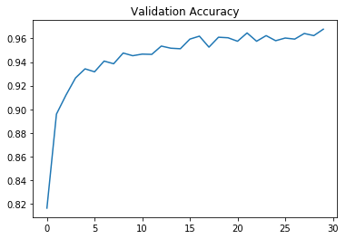
EPOCH 30 ...
Test Accuracy = 0.999
Validation Accuracy = 0.968
Trained Model Saved.
plt.plot(validation_accuracy_figure)
plt.title("Test Accuracy")
plt.show()

plt.plot(validation_accuracy_figure)
plt.title("Validation Accuracy")
plt.show()

with tf.Session() as sess:
    saver.restore(sess, tf.train.latest_checkpoint('.'))

    train_accuracy = evaluate(X_train, y_train)
    print("Train Accuracy = {:.3f}".format(train_accuracy))

    valid_accuracy = evaluate(X_valid, y_valid)
    print("Valid Accuracy = {:.3f}".format(valid_accuracy))

    test_accuracy = evaluate(X_test, y_test)
    print("Test Accuracy = {:.3f}".format(test_accuracy))
INFO:tensorflow:Restoring parameters from ./train_model.ckpt
Train Accuracy = 0.999
Valid Accuracy = 0.968
Test Accuracy = 0.946
4. Test a Model on New Images
4.1 Load the new data
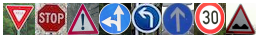
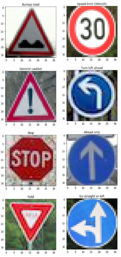
找一些无关的信号灯数据,将数据处理成32×32的大小,用上面训练后保存的模型进行预测:
### Load the images and plot them here.
### Feel free to use as many code cells as needed.
import os
import matplotlib.image as mpimg

dir = "../mydata/"
files = [file for file in os.listdir(dir) if file.endswith('g')]
mydata_x = np.empty((0,32,32,3))
for image_path in files :
    image = mpimg.imread(dir + image_path)
    mydata_x = np.append(mydata_x, np.array([image]), axis=0)
    plt.title(image_path)
    plt.imshow(image)
    plt.show()
将所有图片显示出来。
4.2 Predict the Sign Type for Each Image
csv_data = np.genfromtxt('signnames.csv', delimiter=',', names=True, dtype=None)
sign_names = [t[1].decode('utf-8') for t in csv_data]

my_labels = np.array([22,18, 14, 13, 1, 34, 35,37]) #
with tf.Session() as sess:
    saver.restore(sess, save_file)
    new_pics_classes = sess.run(logits, feed_dict={x: mydata_x, keep_prob : 1.0})
with tf.Session() as sess:
    predicts = sess.run(tf.nn.top_k(new_pics_classes, k=5, sorted=True))

for i in range(len(files)):
    image_path = files[i]
    image = mpimg.imread(dir + image_path)

    # get the predicted label
    class_label = int(predicts[1][i][0])

    plt.title(sign_names[class_label])
    plt.imshow(image)
    plt.show()
将预测的结果,配合label的csv文件,显示预测结果的图片如下:
4.3 Analyze Performance
### Calculate the accuracy for these 5 new images.
### For example, if the model predicted 1 out of 5 signs correctly, it's 20% accurate on these new images.

right_num = 0

for i in range(len(files)):
    class_label = int(predicts[1][i][0])

    right_label = my_labels[i]

    if class_label == right_label:
        right_num += 1

print("New Data Accuracy = ""{:.1%}".format(right_num/len(files)))
New Data Accuracy = 100.0%
4.4 Output Top 5 Softmax Probabilities For Each Image Found on the Web
For each of the new images, print out the model’s softmax probabilities to show the certainty of the model’s predictions (limit the output to the top 5 probabilities for each image). tf.nn.top_k could prove helpful here.
softmax_logits = tf.nn.softmax(logits)
top_k = tf.nn.top_k(softmax_logits, k=3)

with tf.Session() as sess:
    sess.run(tf.global_variables_initializer())
    saver.restore(sess, save_file)
    my_softmax_logits = sess.run(softmax_logits, feed_dict={x: mydata_x, keep_prob: 1.0})
    my_top_k = sess.run(top_k, feed_dict={x: mydata_x, keep_prob: 1.0})

for i in range(len(predicts[0])):
    print("----------------------------------------------------")
    print('Image', i, 'probabilities:', my_top_k[0][i], '\n and predicted classes:', my_top_k[1][i])
    print('and predicted classes label:[',sign_names[my_top_k[1][i][0]],",",sign_names[my_top_k[1][i][1]],",",sign_names[my_top_k[1][i][2]],"]")
输出结果如下:
INFO:tensorflow:Restoring parameters from train_model.ckpt
----------------------------------------------------
Image 0 probabilities: [ 0.9967528  0.0015412  0.0013591]
 and predicted classes: [22 29 26]
and predicted classes label:[ Bumpy road , Bicycles crossing , Traffic signals ]
----------------------------------------------------
Image 1 probabilities: [  1.00000000e+00   1.19113927e-10   2.74432559e-14]
 and predicted classes: [18 27 11]
and predicted classes label:[ General caution , Pedestrians , Right-of-way at the next intersection ]
----------------------------------------------------
Image 2 probabilities: [ 1.  0.  0.]
 and predicted classes: [14  0  1]
and predicted classes label:[ Stop , Speed limit (20km/h) , Speed limit (30km/h) ]
----------------------------------------------------
Image 3 probabilities: [ 1.  0.  0.]
 and predicted classes: [13  0  1]
and predicted classes label:[ Yield , Speed limit (20km/h) , Speed limit (30km/h) ]
----------------------------------------------------
Image 4 probabilities: [  9.99579489e-01   4.18905809e-04   1.32615094e-06]
 and predicted classes: [ 1  2 31]
and predicted classes label:[ Speed limit (30km/h) , Speed limit (50km/h) , Wild animals crossing ]
----------------------------------------------------
Image 5 probabilities: [ 1.  0.  0.]
 and predicted classes: [34  0  1]
and predicted classes label:[ Turn left ahead , Speed limit (20km/h) , Speed limit (30km/h) ]
----------------------------------------------------
Image 6 probabilities: [  9.99985099e-01   7.76796333e-06   5.23519066e-06]
 and predicted classes: [35 25 36]
and predicted classes label:[ Ahead only , Road work , Go straight or right ]
----------------------------------------------------
Image 7 probabilities: [  9.99999642e-01   3.80620122e-07   1.95007988e-09]
 and predicted classes: [37 40 10]
and predicted classes label:[ Go straight or left , Roundabout mandatory , No passing for vehicles over 3.5 metric tons ]
下面是第一个图片的前三位预测结果:
| Probability | Prediction |
|---|---|
| 0.9967528 | Bumpy Road |
| 0.0015 | Bicycles crossing |
| 0.0013 | Traffic signals |
5. 小结
这个项目相对简单,通过对LeNet的改造实现对新数据的训练学习,最后预测完全无关的新数据集。