- 1. Introduction
- 4. Transfer Learning
- 7. AlexNet
- 9. VGG
- 11. Googlenet
- 12. ResNet
- 13. Without Pre-trained Weights
- 14. Lab: Transfer Learning
1. Introduction
深度学习工程师一般并不从头开始搭建神经网络,因为从头搭建没有必要,而且耗时很长,所以更多的时候是修改已有的神经网络,对现有网络进行微调十分有用,这样的过程称为迁移学习。
4. Transfer Learning
迁移学习是指利用一个已经训练完毕的神经网络,微调这个神经网络以适应新的不同的数据集。
一般来说分成下面四个case:
- new data set is small, new data is similar to original training data
- new data set is small, new data is different from original training data
- new data set is large, new data is similar to original training data
- new data set is large, new data is different from original training data
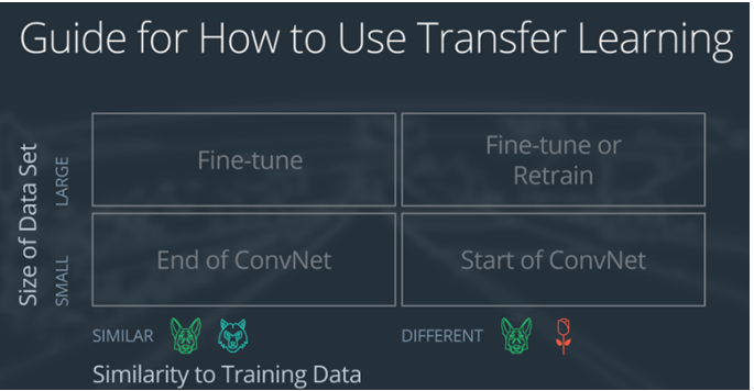
如上图,分别表示了各种case下的处理方式。
假设有下面这样一个神经网络,看看在各种case下该如何训练:
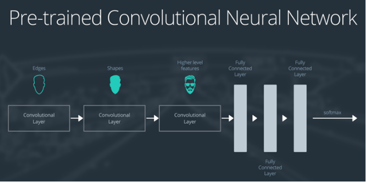
- 第一层卷积检测出图片边界
- 第二层卷积检测出形状
- 第三层卷积检测出更高层次的特征
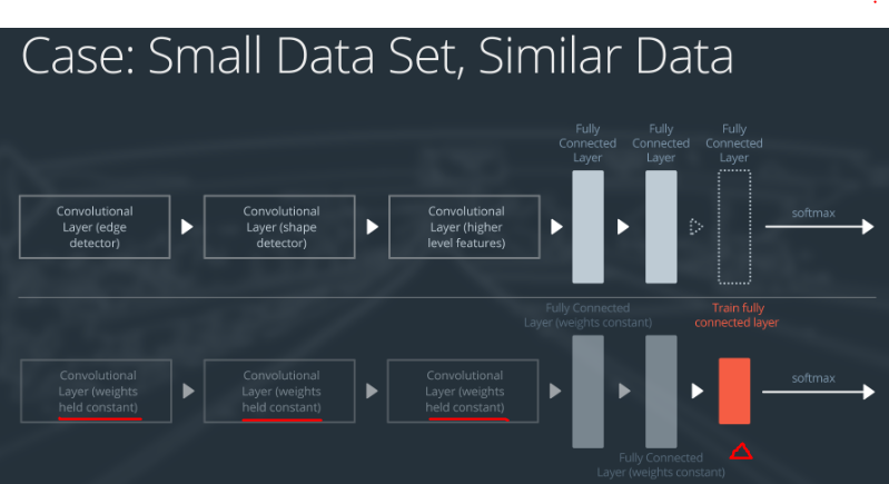
Case 1: Small Data Set, Similar Data
处理方式如下:
- slice off(切开) the end of the neural network
- add a new fully connected layer that matches the number of classes in the new data set
- randomize the weights of the new fully connected layer; freeze all the weights from the pre-trained network
- train the network to update the weights of the new fully connected layer
为了避免对新的小数据集过拟合,神经网络中的权重保持不变,另外,因为新的数据集与既有数据相似,所以大部分训练好的神经网络层的特征,都适用于新的数据集。
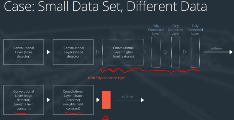
Case 2: Small Data Set, Different Data
处理方式如下:
- slice off most of the pre-trained layers near the beginning of the network
- add to the remaining pre-trained layers a new fully connected layer that matches the number of classes in the new data set
- randomize the weights of the new fully connected layer; freeze all the weights from the pre-trained network
- train the network to update the weights of the new fully connected layer
因为数据量小,所以过拟合仍然是个问题,为了避免过拟合,既有神经网络的权重仍然要保留。
另外,因为数据集的特征不同,所以更高层次的layer可以不要,仅仅使用底层的神经网络layer。
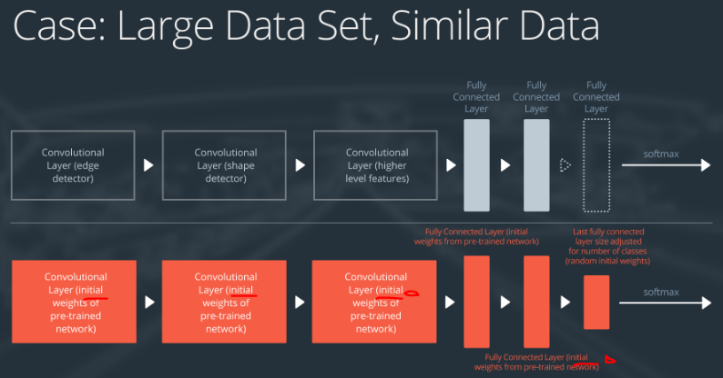
Case 3: Large Data Set, Similar Data
处理方式如下:
- remove the last fully connected layer and replace with a layer matching the number of classes in the new data set
- randomly initialize the weights in the new fully connected layer
- initialize the rest of the weights using the pre-trained weights
- re-train the entire neural network
因为数据量大所以不用担心过拟合问题,可以重新训练权重。另外,因为新数据集与旧数据集有类似的特征,所以之前的神经网络layer保留
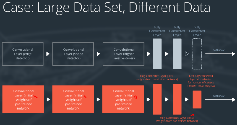
Case 4: Large Data Set, Different Data
处理方式如下:
- remove the last fully connected layer and replace with a layer matching the number of classes in the new data set
- retrain the network from scratch with randomly initialized weights
- alternatively, you could just use the same strategy as the “large and similar” data case
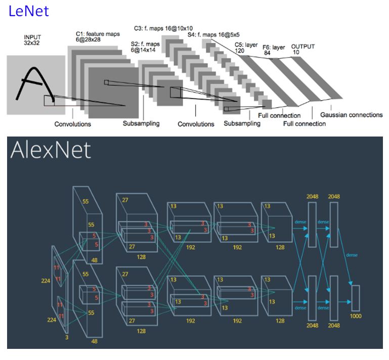
7. AlexNet
相对于LeNet,AlexNet有了如下的改善:
- 利用GPU并行运算的特性,加速了神经网络的训练
- 使用ReLU作为激活函数修正线性单元
- 使用Dropout防止过拟合
9. VGG
VGG模型是2014年ILSVRC竞赛的第二名,第一名是GoogLeNet。但是VGG模型在多个迁移学习任务中的表现要优于googLeNet。而且,从图像中提取CNN特征,VGG模型是首选算法。它的缺点在于,参数量有140M之多,需要更大的存储空间。
GoogLeNet和VGG的Classification模型从原理上并没有与传统的CNN模型有太大不同。大家所用的Pipeline也都是:训练时候:各种数据Augmentation(剪裁,不同大小,调亮度,饱和度,对比度,偏色),剪裁送入CNN模型,Softmax,Backprop。测试时候:尽量把测试数据又各种Augmenting(剪裁,不同大小),把测试数据各种Augmenting后在训练的不同模型上的结果再继续Averaging出最后的结果。
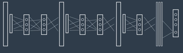
因为VGG结构简单,非常适合迁移学习,主要由一长串3×3大小的卷积层组成,卷积层之间是2×2的池化层,最后是3个全连接层。
VGG in Keras:
Keras中有两个版本的VGG,分别是VGG16和VGG19,对应的layer数量不同。
from keras.applications.vgg16 import VGG16

model = VGG16(weights='imagenet', include_top=False)
上面有两个参数,意思分别是:
- 表示加载imagenet的权重参数
- include_top为false表示不需要使用神经网络最后的一层,在imagenet中有1000个label,一般不需要那么多,所以这里设置false
在imaget神经网络中,数据是经过预处理的,在这里也需要相同的预处理,否则output会出错,VGG使用224×224的图片作为input,所以需要下面的代码:
from keras.preprocessing import image
from keras.applications.vgg16 import preprocess_input
import numpy as np

img_path = 'your_image.jpg'
img = image.load_img(img_path, target_size=(224, 224))
x = image.img_to_array(img)
x = np.expand_dims(x, axis=0)
x = preprocess_input(x)
1. Demo: VGG without Pre-trained Weights
Load example images and pre-process them
# Load our images first, and we'll check what we have
from glob import glob
import matplotlib.image as mpimg
import matplotlib.pyplot as plt
from keras.preprocessing import image
from keras.applications.vgg16 import preprocess_input
import numpy as np

image_paths = glob('images/*.jpg')

i = 2 # Can change this to your desired image to test
img_path = image_paths[i]
img = image.load_img(img_path, target_size=(224, 224))
x = image.img_to_array(img)
x = np.expand_dims(x, axis=0)
x = preprocess_input(x)
Load VGG16 model, but without pre-trained weights
This time, we won’t use the pre-trained weights, so we’ll likely get so wacky predictions.
# Note - this will likely need to download a new version of VGG16
from keras.applications.vgg16 import VGG16, decode_predictions

# Load VGG16 without pre-trained weights
model = VGG16(weights=None)

# Perform inference on our pre-processed image
predictions = model.predict(x)

# Check the top 3 predictions of the model
print('Predicted:', decode_predictions(predictions, top=3)[0])
2. Demo: Using VGG with Keras
Load some example images:
# Load our images first, and we'll check what we have
from glob import glob
import matplotlib.image as mpimg
import matplotlib.pyplot as plt
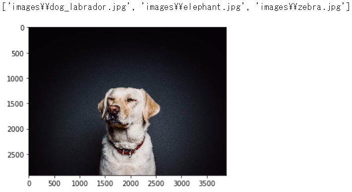
image_paths = glob('images/*.jpg')
# Print out the image paths
print(image_paths)
# View an example of an image
example = mpimg.imread(image_paths[0])
plt.imshow(example)
plt.show()
Pre-process an image
Note that the image.load_img() function will re-size our image to 224x224 as desired for input into this VGG16 model, so the images themselves don’t have to be 224x224 to start.
# Here, we'll load an image and pre-process it
from keras.preprocessing import image
from keras.applications.vgg16 import preprocess_input
import numpy as np

i = 0 # Can change this to your desired image to test
img_path = image_paths[i]
img = image.load_img(img_path, target_size=(224, 224))
x = image.img_to_array(img)
x = np.expand_dims(x, axis=0)
x = preprocess_input(x)
Load VGG16 pre-trained model
We won’t throw out the top fully-connected layer this time when we load the model, as we actually want the true ImageNet-related output. However, you’ll learn how to do this in a later lab. The inference will be a little slower than you might expect here as we are not using GPU just yet.
Note also the use of decode_predictions which will map the prediction to the class name.
# Note - this will likely need to download a new version of VGG16
from keras.applications.vgg16 import VGG16, decode_predictions

# Load the pre-trained model
model = VGG16(weights='imagenet')

# Perform inference on our pre-processed image
predictions = model.predict(x)

# Check the top 3 predictions of the model
print('Predicted:', decode_predictions(predictions, top=3)[0])
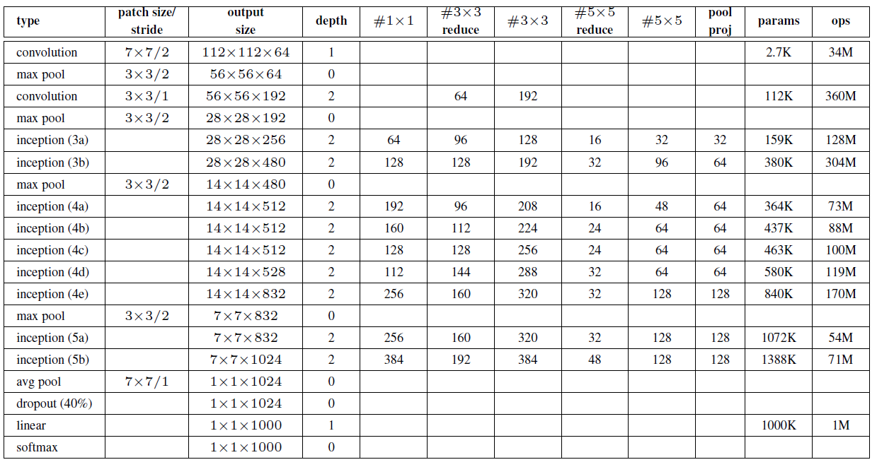
11. Googlenet
GoogLeNet是2014年Christian Szegedy提出的一种全新的深度学习结构,在这之前的AlexNet、VGG等结构都是通过增大网络的深度(层数)来获得更好的训练效果,但层数的增加会带来很多负作用,比如overfit、梯度消失、梯度爆炸等。inception的提出则从另一种角度来提升训练结果:能更高效的利用计算资源,在相同的计算量下能提取到更多的特征,从而提升训练结果。
采用Inception架构的GoogLeNet如下所示:
同样在Keras中的实现代码为:
from keras.applications.inception_v3 import InceptionV3

model = InceptionV3(weights='imagenet', include_top=False)
一样的需要进行数据预处理,不过这里不同的是,InceptionV3使用299*299的input图片。
12. ResNet
Imagenet2015年微软使用的网络,将图片的识别错误率降低到了3%,其主要特点是高达152层的网络。对比下层数:
| 网络 | 层数 |
|---|---|
| ResNet | 152 |
| AlexNet | 8 |
| VGG | 19 |
| GoogleNet | 22 |
其在代码中的实现为:
from keras.applications.resnet50 import ResNet50

model = ResNet50(weights='imagenet', include_top=False)
图片input的大小要处理为224*224.
13. Without Pre-trained Weights
1. Demo: VGG without Pre-trained Weights
Load example images and pre-process them
# Load our images first, and we'll check what we have
from glob import glob
import matplotlib.image as mpimg
import matplotlib.pyplot as plt
from keras.preprocessing import image
from keras.applications.vgg16 import preprocess_input
import numpy as np

image_paths = glob('images/*.jpg')

i = 2 # Can change this to your desired image to test
img_path = image_paths[i]
img = image.load_img(img_path, target_size=(224, 224))
x = image.img_to_array(img)
x = np.expand_dims(x, axis=0)
x = preprocess_input(x)
Load VGG16 model, but without pre-trained weights
This time, we won’t use the pre-trained weights, so we’ll likely get so wacky predictions.
# Note - this will likely need to download a new version of VGG16
from keras.applications.vgg16 import VGG16, decode_predictions

# Load VGG16 without pre-trained weights
model = VGG16(weights=None)

# Perform inference on our pre-processed image
predictions = model.predict(x)

# Check the top 3 predictions of the model
print('Predicted:', decode_predictions(predictions, top=3)[0])
2. Demo: Using VGG with Keras
Load some example images:
# Load our images first, and we'll check what we have
from glob import glob
import matplotlib.image as mpimg
import matplotlib.pyplot as plt

image_paths = glob('images/*.jpg')

# Print out the image paths
print(image_paths)

# View an example of an image
example = mpimg.imread(image_paths[0])
plt.imshow(example)
plt.show()
Pre-process an image
Note that the image.load_img() function will re-size our image to 224x224 as desired for input into this VGG16 model, so the images themselves don’t have to be 224x224 to start.
# Here, we'll load an image and pre-process it
from keras.preprocessing import image
from keras.applications.vgg16 import preprocess_input
import numpy as np

i = 0 # Can change this to your desired image to test
img_path = image_paths[i]
img = image.load_img(img_path, target_size=(224, 224))
x = image.img_to_array(img)
x = np.expand_dims(x, axis=0)
x = preprocess_input(x)
Load VGG16 pre-trained model
We won’t throw out the top fully-connected layer this time when we load the model, as we actually want the true ImageNet-related output. However, you’ll learn how to do this in a later lab. The inference will be a little slower than you might expect here as we are not using GPU just yet.
Note also the use of decode_predictions which will map the prediction to the class name.
# Note - this will likely need to download a new version of VGG16
from keras.applications.vgg16 import VGG16, decode_predictions

# Load the pre-trained model
model = VGG16(weights='imagenet')

# Perform inference on our pre-processed image
predictions = model.predict(x)

# Check the top 3 predictions of the model
print('Predicted:', decode_predictions(predictions, top=3)[0])
14. Lab: Transfer Learning
本节使用一个ImageNet中训练好的神经网络和权重,去微调出另一个神经网络,在这里需要:
- 添加新的网络层
- 冻结权重
14.1 GPU usage
在这里我们使用googlet的inception v3,另外需要将input_shape修改为139*139*3,另外因为最终的output不同,所以将include_top 设为 False,这意味着最后的一个全连接层(有1000个node),以及一个全局的Average池化层被drop掉了。
# Set a couple flags for training - you can ignore these for now
freeze_flag = True  # `True` to freeze layers, `False` for full training
weights_flag = 'imagenet' # 'imagenet' or None
preprocess_flag = True # Should be true for ImageNet pre-trained typically

# Loads in InceptionV3
from keras.applications.inception_v3 import InceptionV3

# We can use smaller than the default 299x299x3 input for InceptionV3
# which will speed up training. Keras v2.0.9 supports down to 139x139x3
input_size = 139

# Using Inception with ImageNet pre-trained weights
inception = InceptionV3(weights=weights_flag, include_top=False,
                        input_shape=(input_size,input_size,3))
14.2 Pre-trained with frozen weights
You can freeze layers by setting layer.trainable to False for a given layer. Within a model, you can get the list of layers with model.layers.
if freeze_flag == True:
    ## TODO: Iterate through the layers of the Inception model
    ##       loaded above and set all of them to have trainable = False
    for layer in inception.layers:
        layer.trainable = False
14.3 Dropping layers
You can drop layers from a model with model.layers.pop(). Before you do this, you should check out what the actual layers of the model are with Keras’s .summary() function.
## TODO: Use the model summary function to see all layers in the
##       loaded Inception model
inception.summary()
一个通常的inception网络,可以看到最后的两层分别是全局的平均池化层和全连接Dense层,因为这里设置了include_top为Flase,所以这两个layer被drop掉了,如果还需要额外drop其他层,可以使用inception.layers.pop()。
14.4 Adding new layers
之前使用Sequential模型的时候,我们使用model.add()来添加layer,在这里使用不同的方法,显式的将一个层attach到当前层后面。比如,如果要在inp这个层后面添加drop层,使用:x = Dropout(0.2)(inp)
from keras.layers import Input, Lambda
import tensorflow as tf

# Makes the input placeholder layer 32x32x3 for CIFAR-10
cifar_input = Input(shape=(32,32,3))

# Re-sizes the input with Kera's Lambda layer & attach to cifar_input
resized_input = Lambda(lambda image: tf.image.resize_images(
    image, (input_size, input_size)))(cifar_input)

# Feeds the re-sized input into Inception model
# You will need to update the model name if you changed it earlier!
inp = inception(resized_input)
相同的方法,再添加一个全局池化层和全连接层:
# Imports fully-connected "Dense" layers & Global Average Pooling
from keras.layers import Dense, GlobalAveragePooling2D

## TODO: Setting `include_top` to False earlier also removed the
##       GlobalAveragePooling2D layer, but we still want it.
##       Add it here, and make sure to connect it to the end of Inception
x = GlobalAveragePooling2D()(inp)

## TODO: Create two new fully-connected layers using the Model API
##       format discussed above. The first layer should use `out`
##       as its input, along with ReLU activation. You can choose
##       how many nodes it has, although 512 or less is a good idea.
##       The second layer should take this first layer as input, and
##       be named "predictions", with Softmax activation and
##       10 nodes, as we'll be using the CIFAR10 dataset.
x = Dense(512, activation = 'relu')(x)
predictions = Dense(10, activation = 'softmax')(x)
# Imports the Model API
from keras.models import Model

# Creates the model, assuming your final layer is named "predictions"
model = Model(inputs=cifar_input, outputs=predictions)

# Compile the model
model.compile(optimizer='Adam', loss='categorical_crossentropy', metrics=['accuracy'])

# Check the summary of this new model to confirm the architecture
model.summary()
如下就生成了一个新的网络,注意之前被冻结的网络,在下面用一行显式了inception_v3 (Model) :
Layer (type)                 Output Shape              Param #
=================================================================
input_2 (InputLayer)         (None, 32, 32, 3)         0
_________________________________________________________________
lambda_1 (Lambda)            (None, 139, 139, 3)       0
_________________________________________________________________
inception_v3 (Model)         (None, 3, 3, 2048)        21802784
_________________________________________________________________
global_average_pooling2d_1 ( (None, 2048)              0
_________________________________________________________________
dense_1 (Dense)              (None, 512)               1049088
_________________________________________________________________
dense_2 (Dense)              (None, 10)                5130
=================================================================
Total params: 22,857,002
Trainable params: 1,054,218
Non-trainable params: 21,802,784
_________________________________________________________________
14.5 GPU time
The rest of the notebook will give you the code for training, so you can turn on the GPU at this point - but first, make sure to save your jupyter notebook. Once the GPU is turned on, it will load whatever your last notebook checkpoint is.
While we suggest reading through the code below to make sure you understand it, you can otherwise go ahead and select Cell > Run All (or Kernel > Restart & Run All if already using GPU) to run through all cells in the notebook.
from sklearn.utils import shuffle
from sklearn.preprocessing import LabelBinarizer
from keras.datasets import cifar10

(X_train, y_train), (X_val, y_val) = cifar10.load_data()

# One-hot encode the labels
label_binarizer = LabelBinarizer()
y_one_hot_train = label_binarizer.fit_transform(y_train)
y_one_hot_val = label_binarizer.fit_transform(y_val)

# Shuffle the training & test data
X_train, y_one_hot_train = shuffle(X_train, y_one_hot_train)
X_val, y_one_hot_val = shuffle(X_val, y_one_hot_val)

# We are only going to use the first 10,000 images for speed reasons
# And only the first 2,000 images from the test set
X_train = X_train[:10000]
y_one_hot_train = y_one_hot_train[:10000]
X_val = X_val[:2000]
y_one_hot_val = y_one_hot_val[:2000]
# Use a generator to pre-process our images for ImageNet
from keras.preprocessing.image import ImageDataGenerator
from keras.applications.inception_v3 import preprocess_input

if preprocess_flag == True:
    datagen = ImageDataGenerator(preprocessing_function=preprocess_input)
    val_datagen = ImageDataGenerator(preprocessing_function=preprocess_input)
else:
    datagen = ImageDataGenerator()
    val_datagen = ImageDataGenerator()
# Train the model
batch_size = 32
epochs = 5
# Note: we aren't using callbacks here since we only are using 5 epochs to conserve GPU time
model.fit_generator(datagen.flow(X_train, y_one_hot_train, batch_size=batch_size),
                    steps_per_epoch=len(X_train)/batch_size, epochs=epochs, verbose=1,
                    validation_data=val_datagen.flow(X_val, y_one_hot_val, batch_size=batch_size),
                    validation_steps=len(X_val)/batch_size)
14.6 Test without frozen weights, or by training from scratch
上面使用了ImageNet中的权值,所以速度比较快,如果不将其冻结的话,将freeze_flag设置为False。
另外,如果不使用ImageNet中的预置权值从头开始训练的话,将weights_flag 设定为None。
上面三种case,最后的GPU使用时间对比为:
| Training Mode | Val Acc @ 1 epoch | Val Acc @ 5 epoch | Time per epoch |
|---|---|---|---|
| Frozen weights | 65.5% | 70.3% | 50 seconds |
| Unfrozen weights | 50.6% | 71.6% | 142 seconds |
| No pre-trained weights | 19.2% | 39.2% | 142 seconds |