- 0. 小结
- 2. Intro
- 3. Lesson Map and Fusion Flow
- 4. Lesson Variables and Equations
- 5. Estimation Problem Refresh
- 6. Kalman Filter Intuition
- 7. Kalman Filter Equations in C++ Part 1
- 9. State Prediction
- 10. Process Covariance Matrix(协方差)
- 11. Laser Measurements Part 1
- 13. Laser Measurements Part 3
- 14. Laser Measurements Part 4
- 15. Radar Measurements
- 16. Mapping with a Nonlinear Function
- 17. Extended Kalman Filter
- 18. Multivariate Taylor Series Expansion
- 19. Jacobian Matrix Part 1
- 21. EKF Algorithm Generalization
- 22. Sensor Fusion General Flow
- 23. Evaluating KF Performance Part 1
- 25. Outro
- 26. Bonus Round: Sensor Fusion [Optional]
0. 小结
本章主要讲扩展的卡尔曼滤波器,这种扩展卡尔曼滤波器能够处理不同类型的数据,如雷达和激光雷达,由于雷达数据不同于激光雷达,当接收数据是雷达时,需要使用不同的预测和更新方式,最后描述了如何评价估算结果的方式,所有的方法都有对应C++代码。
- 参考:
- EKF Tutorial 浅显易懂的扩展滤波器介绍,而且带有交互式的程序可以确认效果
2. Intro
本模块的实战项目计划,是利用传感器融合追踪一名行人。将激光雷达和雷达的优势劣势结合起来,一起来估算行人位置,方向和速度。这些功能都是在C++中实现。
3. Lesson Map and Fusion Flow
本章中将所有学习到的知识结合起来,开发一个完整的融合模型,基于卡尔曼滤波器的融合包括很多方面。 首先需要创建一个扩展卡尔曼滤波器,扩展的意思是它能处理更复杂的运动模型和测量模型。下面是整体的处理流程:
- 首先是两个传感器,激光雷达和雷达,它们提供信息用于估算移动中行人的状态。状态通过二维位置和二维速度表示。
- 每次收到特定传感器的新测量值时,都会触发估算函数,估算函数中,我们执行两个步骤,状态预测和测量更新。
- 在预测步骤中,我们在协方差中预测行人状态。具体做法是,考虑当前和前一次观察之间的时间差。
- 在测量更新中,将取决于传感器类型,如果当前数据来自激光传感器,我们可以应用一个标准的通用滤波器来更新行人状态。雷达测量值需要使用非线性测量函数。因为我们收到雷达测量值时,会使用不同的方法来处理测量更新,比如,我们可能使用扩展滤波器方程。

卡尔曼滤波算法包含如下的步骤:
- 首次测量:滤波器将接收自行车相对于汽车位置的初始测量值,这个测量值来自于激光雷达或是雷达。
- 初始状态和其协方差矩阵:滤波器基于首次测量值,初始化自行车的位置。
- 然后在一定时间间隔Δt后,汽车收到另一个传感器测量值。
- 预测:算法将预测在时间Δt后,自行车的位置。一个基础的方式是假设自行车是匀速的。
- 更新:滤波器比较预测的位置,以及传感器的测量值,得到一个更新后的位置。这时用到的就是卡尔曼滤波器算法。
4. Lesson Variables and Equations
the derivations of the Kalman Filter equations
5. Estimation Problem Refresh
我们要追踪在无人驾驶车前移动的行人,通用滤波器时一个两步估算问题,预测与更新。
- 开始时,我们依赖已知的行人信息,推断出行人在下次测量到达时的行人状态,这叫做预测步骤。
- 下一步是更,使用新的观察数据纠正我们对于行人状态的推测值。

如果有多个测量值呢,即多个传感器同时进行测量:

实际上也是相同的流程,如上图。

- MEAN(X):是一个状态矩阵,包含了需要跟踪物体的位置和速度(velocity)
- P:是状态的协方差矩阵,包含了物体的位置和速度的不确定性信息
- k:表示时间跨度
-
k+1 k : 表示预测步骤的值 - Xk,Pk : 表示经过更新后的值
6. Kalman Filter Intuition
本节是对卡尔曼滤波的详解,可以参考卡尔曼滤波器最佳线性滤波器原理
下面是预测更新流程:

卡尔曼滤波的预测与更新公式:

预测:
上面左侧的预测公式:
- F表示状态迁移矩阵,v表示加速度减速度等不确定性因为在这段时间内产生的不确定性。x表示前一个时间段的位置和速度状态,x’表示预测的下一个时间段状态。
- P表示状态的协方差矩阵,即这个预测所产生的不确定性,FPF(T)表示迁移过来的协方差,后面的Q表示预测模型本身带来的噪声。
更新:
y=z−Hx',y表示观测本身带来的噪声,z表示观测值- K矩阵,通常也叫做卡尔曼滤波增量,它结合了预测带来的噪声P’和测量传感器的噪声R,这个矩阵可以根据噪声P和R的大小,调整到底相信预测多一点,还是相信测量值多一点。
7. Kalman Filter Equations in C++ Part 1
后面的练习中,使用到一个库 Eigen Library,参考资料here
常见使用方法的示例代码如下:
#include "Eigen/Dense"

VectorXd my_vector(2);
my_vector << 10, 20;
cout << my_vector << endl;

MatrixXd my_matrix(2,2);
my_matrix << 1, 2,
             3, 4;

my_matrix(1,0) = 11;    //second row, first column
my_matrix(1,1) = 12;    //second row, second column

MatrixXd my_matrix_t = my_matrix.transpose();
MatrixXd my_matrix_i = my_matrix.inverse();

MatrixXd another_matrix;
another_matrix = my_matrix*my_vector;
/**
 * Write a function 'filter()' that implements a multi-
 *   dimensional Kalman Filter for the example given
 */

#include <iostream>
#include <vector>
#include "Dense"

using std::cout;
using std::endl;
using std::vector;
using Eigen::VectorXd;
using Eigen::MatrixXd;

// Kalman Filter variables
VectorXd x;	// object state
MatrixXd P;	// object covariance matrix
VectorXd u;	// external motion
MatrixXd F; // state transition matrix
MatrixXd H;	// measurement matrix
MatrixXd R;	// measurement covariance matrix
MatrixXd I; // Identity matrix
MatrixXd Q;	// process covariance matrix

vector<VectorXd> measurements;
void filter(VectorXd &x, MatrixXd &P);


int main() {
  /**
   * Code used as example to work with Eigen matrices
   */
  // design the KF with 1D motion
  x = VectorXd(2);
  x << 0, 0;

  P = MatrixXd(2, 2);
  P << 1000, 0, 0, 1000;

  u = VectorXd(2);
  u << 0, 0;

  F = MatrixXd(2, 2);
  F << 1, 1, 0, 1;

  H = MatrixXd(1, 2);
  H << 1, 0;

  R = MatrixXd(1, 1);
  R << 1;

  I = MatrixXd::Identity(2, 2);

  Q = MatrixXd(2, 2);
  Q << 0, 0, 0, 0;

  // create a list of measurements
  VectorXd single_meas(1);
  single_meas << 1;
  measurements.push_back(single_meas);
  single_meas << 2;
  measurements.push_back(single_meas);
  single_meas << 3;
  measurements.push_back(single_meas);

  // call Kalman filter algorithm
  filter(x, P);

  return 0;
}


void filter(VectorXd &x, MatrixXd &P) {

  for (unsigned int n = 0; n < measurements.size(); ++n) {

    VectorXd z = measurements[n];
    // TODO: YOUR CODE HERE
    /**
     * KF Measurement update step
     */
    VectorXd y = z - H * x; // 新测量值z时的误差计算
    MatrixXd Ht = H.transpose(); //h矩阵转置
    MatrixXd S = H * P * Ht + R; //s矩阵
    MatrixXd Si = S.inverse(); //s矩阵的求逆矩阵
    MatrixXd K =  P * Ht * Si; //卡尔曼增益

    // new state
    x = x + (K * y); //预测后的状态
    P = (I - K * H) * P; //预测后的协方差

    /**
     * KF Prediction step
     */
    x = F * x + u;
    MatrixXd Ft = F.transpose();
    P = F * P * Ft + Q;

    cout << "x=" << endl <<  x << endl;
    cout << "P=" << endl <<  P << endl;
  }
}
输出:
x=
0.999001
       0
P=
1001 1000
1000 1000
x=
   2.998
0.999002
P=
4.99002 2.99302
2.99302 1.99501
x=
3.99967
      1
P=
 2.33189 0.999168
0.999168 0.499501
参考代码(python)here
def kalman_filter(x, P):
    print(x)
    for n in range(len(measurements)):
        # measurement update
        Z = matrix([[measurements[n]]])
        y = Z - (H * x)
        S = H * P * H.transpose()  + R
        K = P * H.transpose() * S.inverse()
        P = (I - (K*H)) * P

        x = x + (K * y)

        # prediction
        P = F * P * F.transpose()
        x = (F*x) + u
    return x,P
9. State Prediction
上面用C++实现了一个卡尔曼滤波器来预测更新一维数据,现在驾驶传感器提供的是二维测量数据。

还有一点与之前不同,就是时间差不是固定的了:

x'=Fx+noise 中noise是指在预测位置时产生得不确定性,模型假设在一定间隔内是匀速的,但是实际上物体可能加速减速,那这个模型就通过noise来表示这种不确定性。
测量误差也是存在的,表示传感器测量带来的不确定性。
Quiz1:比较时间间隔0.1秒,和时间间隔5秒,哪个产生的不确定性高,显然是5秒产生的不确定性更大,可以简单的将5秒分成50个0.1秒,而且这连续的50个0.1s中没有反馈可以纠正数据,那么5秒的不确定性,也就是噪声显然是大于0.1秒。 Quiz2:一个行人在一段时间内,有加速有减速,有停止,那这个会给预测模型带来很大的噪声。
From the examples I’ve just showed you we can clearly see that the process noise depends on both:
- the elapsed time
- the uncertainty of acceleration.
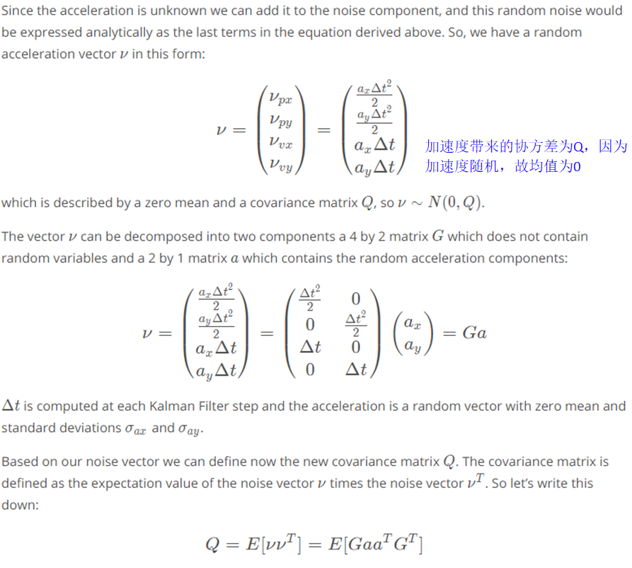
10. Process Covariance Matrix(协方差)
最终状态更新的时候,我们需要将处理(预测时)协方差矩阵转换成状态协方差矩阵。
下面是处理协方差矩阵的计算过程:


更加详细推导过程参考下图:


11. Laser Measurements Part 1
这里需要将预测得到的状态向量,转换为测量得到的位置向量,状态向量中有4维度分别是x和y方向上的位置,以及速度,位置向量就是x和y方向的位置。

H是一个观测向量,用于将二维的x状态向量,转换成与z一样的标量(1*p + 0*v得到位置p,z也是位置信息)。
13. Laser Measurements Part 3

R表示测量的协方差矩阵,用于衡量接收到 激光传感器位置值的不确定性。
下面的编程练习中,实现一个卡尔曼滤波器,该滤波器可以代入激光雷达测量值,并在二维平面上追踪行人,如下图中,行人的状态由右边的state vector表示:

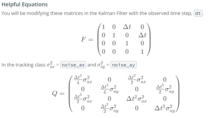
代码主要分为三个类:kalman_filter,tracking,measurement_package。在这个练习中,需要根据当前和之前的测量值之间的时间差,修改F和Q的矩阵。

最后添加的代码在tracking类中的ProcessMeasurement函数中。
13.1 main.cpp
#include <iostream>
#include <sstream>
#include <vector>
#include "Dense"
#include "measurement_package.h"
#include "tracking.h"

using Eigen::MatrixXd;
using Eigen::VectorXd;
using std::cout;
using std::endl;
using std::ifstream;
using std::istringstream;
using std::string;
using std::vector;


int main() {

  /**
   * Set Measurements
   */
  vector<MeasurementPackage> measurement_pack_list;

  // hardcoded input file with laser and radar measurements
  string in_file_name_ = "obj_pose-laser-radar-synthetic-input.txt";
  ifstream in_file(in_file_name_.c_str(), ifstream::in);

  if (!in_file.is_open()) {
    cout << "Cannot open input file: " << in_file_name_ << endl;
  }

  string line;
  // set i to get only first 3 measurments
  int i = 0;
  while (getline(in_file, line) && (i<=3)) {

    MeasurementPackage meas_package;

    istringstream iss(line);
    string sensor_type;
    iss >> sensor_type; // reads first element from the current line
    int64_t timestamp;
    if (sensor_type.compare("L") == 0) {  // laser measurement
      // read measurements
      meas_package.sensor_type_ = MeasurementPackage::LASER;
      meas_package.raw_measurements_ = VectorXd(2);
      float x;
      float y;
      iss >> x;
      iss >> y;
      meas_package.raw_measurements_ << x,y;
      iss >> timestamp;
      meas_package.timestamp_ = timestamp;
      measurement_pack_list.push_back(meas_package);

    } else if (sensor_type.compare("R") == 0) {
      // Skip Radar measurements
      continue;
    }
    ++i;
  }

  // Create a Tracking instance
  Tracking tracking;

  // call the ProcessingMeasurement() function for each measurement
  size_t N = measurement_pack_list.size();
  // start filtering from the second frame
  // (the speed is unknown in the first frame)
  for (size_t k = 0; k < N; ++k) {
    tracking.ProcessMeasurement(measurement_pack_list[k]);
  }

  if (in_file.is_open()) {
    in_file.close();
  }
  return 0;
}
13.2 kalman_filter.cpp
#include "kalman_filter.h"

KalmanFilter::KalmanFilter() {
}

KalmanFilter::~KalmanFilter() {
}

void KalmanFilter::Predict() {
  x_ = F_ * x_;
  MatrixXd Ft = F_.transpose();
  P_ = F_ * P_ * Ft + Q_;
}

void KalmanFilter::Update(const VectorXd &z) {
  VectorXd z_pred = H_ * x_;
  VectorXd y = z - z_pred;
  MatrixXd Ht = H_.transpose();
  MatrixXd S = H_ * P_ * Ht + R_;
  MatrixXd Si = S.inverse();
  MatrixXd PHt = P_ * Ht;
  MatrixXd K = PHt * Si;

  //new estimate
  x_ = x_ + (K * y);
  long x_size = x_.size();
  MatrixXd I = MatrixXd::Identity(x_size, x_size);
  P_ = (I - K * H_) * P_;
}
13.3 kalman_filter.h
#ifndef KALMAN_FILTER_H_
#define KALMAN_FILTER_H_

#include "Dense"

using Eigen::MatrixXd;
using Eigen::VectorXd;

class KalmanFilter {
 public:

  /**
   * Constructor
   */
  KalmanFilter();

  /**
   * Destructor
   */
  virtual ~KalmanFilter();

  /**
   * Predict Predicts the state and the state covariance
   *   using the process model
   */
  void Predict();

  /**
   * Updates the state and
   * @param z The measurement at k+1
   */
  void Update(const VectorXd &z);

  // state vector
  VectorXd x_;

  // state covariance matrix
  MatrixXd P_;

  // state transistion matrix
  MatrixXd F_;

  // process covariance matrix
  MatrixXd Q_;

  // measurement matrix
  MatrixXd H_;

  // measurement covariance matrix
  MatrixXd R_;

};

#endif  // KALMAN_FILTER_H_
13.4 tracking.cpp - 修改后的代码
#include "tracking.h"
#include <iostream>
#include "Dense"
#include <cmath>

using Eigen::MatrixXd;
using Eigen::VectorXd;
using std::cout;
using std::endl;
using std::vector;

Tracking::Tracking() {
  is_initialized_ = false;
  previous_timestamp_ = 0;

  // create a 4D state vector, we don't know yet the values of the x state
  kf_.x_ = VectorXd(4);

  // state covariance matrix P
  kf_.P_ = MatrixXd(4, 4);
  kf_.P_ << 1, 0, 0, 0,
            0, 1, 0, 0,
            0, 0, 1000, 0,
            0, 0, 0, 1000;


  // measurement covariance
  kf_.R_ = MatrixXd(2, 2);
  kf_.R_ << 0.0225, 0,
            0, 0.0225;

  // measurement matrix
  kf_.H_ = MatrixXd(2, 4);
  kf_.H_ << 1, 0, 0, 0,
            0, 1, 0, 0;

  // the initial transition matrix F_
  kf_.F_ = MatrixXd(4, 4);
  kf_.F_ << 1, 0, 1, 0,
            0, 1, 0, 1,
            0, 0, 1, 0,
            0, 0, 0, 1;

  // set the acceleration noise components
  noise_ax = 5;
  noise_ay = 5;
}

Tracking::~Tracking() {

}

// Process a single measurement
void Tracking::ProcessMeasurement(const MeasurementPackage &measurement_pack) {
  if (!is_initialized_) {
    //cout << "Kalman Filter Initialization " << endl;

    // set the state with the initial location and zero velocity
    kf_.x_ << measurement_pack.raw_measurements_[0],
              measurement_pack.raw_measurements_[1],
              0,
              0;

    previous_timestamp_ = measurement_pack.timestamp_;
    is_initialized_ = true;
    return;
  }

  // compute the time elapsed between the current and previous measurements
  // dt - expressed in seconds
  float dt = (measurement_pack.timestamp_ - previous_timestamp_) / 1000000.0;
  previous_timestamp_ = measurement_pack.timestamp_;

  // TODO: YOUR CODE HERE
  // 1. Modify the F matrix so that the time is integrated
  // 2. Set the process covariance matrix Q
  // 3. Call the Kalman Filter predict() function
  // 4. Call the Kalman Filter update() function
  //      with the most recent raw measurements_

   // TODO: YOUR CODE HERE
  float dt_2 = dt * dt;
  float dt_3 = dt_2 * dt;
  float dt_4 = dt_3 * dt;

  // Modify the F matrix so that the time is integrated
  kf_.F_(0, 2) = dt;
  kf_.F_(1, 3) = dt;

  // set the process covariance matrix Q
  kf_.Q_ = MatrixXd(4, 4);
  kf_.Q_ <<  dt_4/4*noise_ax, 0, dt_3/2*noise_ax, 0,
         0, dt_4/4*noise_ay, 0, dt_3/2*noise_ay,
         dt_3/2*noise_ax, 0, dt_2*noise_ax, 0,
         0, dt_3/2*noise_ay, 0, dt_2*noise_ay;

  // predict
  kf_.Predict();

  // measurement update
  kf_.Update(measurement_pack.raw_measurements_);
  cout << "x_= " << kf_.x_ << endl;
  cout << "P_= " << kf_.P_ << endl;
}
13.5 tracking.h
#ifndef TRACKING_H_
#define TRACKING_H_

#include <vector>
#include <string>
#include <fstream>
#include "kalman_filter.h"
#include "measurement_package.h"

class Tracking {
 public:
  Tracking();
  virtual ~Tracking();
  void ProcessMeasurement(const MeasurementPackage &measurement_pack);
  KalmanFilter kf_;

 private:
  bool is_initialized_;
  int64_t previous_timestamp_;

  //acceleration noise components
  float noise_ax;
  float noise_ay;

};

#endif  // TRACKING_H_
13.6 measurement_package.h
#ifndef MEASUREMENT_PACKAGE_H_
#define MEASUREMENT_PACKAGE_H_

#include "Dense"

class MeasurementPackage {
 public:

  enum SensorType {
    LASER, RADAR
  } sensor_type_;

  Eigen::VectorXd raw_measurements_;

  int64_t timestamp_;

};

#endif  // MEASUREMENT_PACKAGE_H_
最后输出:
x_=  0.96749
0.405862
 4.58427
-1.83232
P_= 0.0224541         0  0.204131         0
        0 0.0224541         0  0.204131
 0.204131         0   92.7797         0
        0  0.204131         0   92.7797
x_= 0.958365
0.627631
0.110368
 2.04304
P_= 0.0220006         0  0.210519         0
        0 0.0220006         0  0.210519
 0.210519         0   4.08801         0
        0  0.210519         0   4.08801
x_=   1.34291
 0.364408
  2.32002
-0.722813
P_= 0.0185328         0  0.109639         0
        0 0.0185328         0  0.109639
 0.109639         0   1.10798         0
        0  0.109639         0   1.10798
14. Laser Measurements Part 4
使用公式:
更新的代码如下:
// Process a single measurement
void Tracking::ProcessMeasurement(const MeasurementPackage &measurement_pack) {
  if (!is_initialized_) {
    //cout << "Kalman Filter Initialization " << endl;

    // set the state with the initial location and zero velocity
    kf_.x_ << measurement_pack.raw_measurements_[0],
              measurement_pack.raw_measurements_[1],
              0,
              0;

    previous_timestamp_ = measurement_pack.timestamp_;
    is_initialized_ = true;
    return;
  }

  // compute the time elapsed between the current and previous measurements
  // dt - expressed in seconds
  float dt = (measurement_pack.timestamp_ - previous_timestamp_) / 1000000.0;
  previous_timestamp_ = measurement_pack.timestamp_;

    // TODO: YOUR CODE HERE
  float dt_2 = dt * dt;
  float dt_3 = dt_2 * dt;
  float dt_4 = dt_3 * dt;

  // Modify the F matrix so that the time is integrated
  kf_.F_(0, 2) = dt;
  kf_.F_(1, 3) = dt;

  // set the process covariance matrix Q
  kf_.Q_ = MatrixXd(4, 4);
  kf_.Q_ <<  dt_4/4*noise_ax, 0, dt_3/2*noise_ax, 0,
         0, dt_4/4*noise_ay, 0, dt_3/2*noise_ay,
         dt_3/2*noise_ax, 0, dt_2*noise_ax, 0,
         0, dt_3/2*noise_ay, 0, dt_2*noise_ay;

  // predict
  kf_.Predict();

  // measurement update
  kf_.Update(measurement_pack.raw_measurements_);

  cout << "x_= " << kf_.x_ << endl;
  cout << "P_= " << kf_.P_ << endl;
}
15. Radar Measurements

上面的14节的例子中,只有一个激光雷达,激光雷达只能探测到位置信息,雷达虽然精度不高,但是能获取速度信息,将这两者融合能得到更高的精度。
下面是雷达获取的测量值,与激光雷达不同,包含了:
- 径向距离
- 方向角
- 径向速度

利用卡尔曼滤波器公式:

h(x’)将预测向量,转换成测量向量的形式:
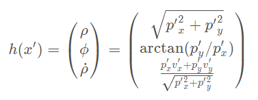
这个函数是个非线性函数,将预测值的位置和速度(笛卡尔坐标),转换成极坐标系(径向半径,径向速度,方向角)的形式。
详细的推导过程如下:


16. Mapping with a Nonlinear Function
What happens if we have a nonlinear measurement function, h(x). Can we apply the Kalman Filter equations to update the predicted state, X, with new measurements, z?
问题:能使用卡尔曼滤波器,来更新测量值z和预测值X吗?
Answer:No, We aren’t working with Gaussian distributions after applying a nonlinear measurement function. 还需要对非线性处理结果进行高斯分布处理。
17. Extended Kalman Filter
如上所述,应用h(x’)函数后,就不是高斯分布了,那么卡尔曼滤波器也不再适用了。
如下图,高斯分布的值,在经过h(x’)函数后:

所以需要对h(x)函数进行线性化操作,这个是扩展卡尔曼滤波器的核心思想。
扩展卡尔曼滤波器使用了一阶泰勒展开法,将非线性函数进行线性化处理。
关于泰勒展开式,参考here
18. Multivariate Taylor Series Expansion

上面的函数,在mu=0处的一阶泰勒展开式 h(x)≈x。

19. Jacobian Matrix Part 1

Hj矩阵形式为:
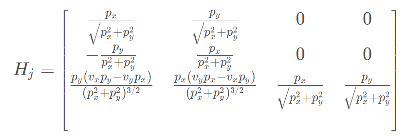
用代码实现为:
#include <iostream>
#include <vector>
#include "Dense"

using Eigen::MatrixXd;
using Eigen::VectorXd;
using std::cout;
using std::endl;

MatrixXd CalculateJacobian(const VectorXd& x_state);

int main() {
  /**
   * Compute the Jacobian Matrix
   */

  // predicted state example
  // px = 1, py = 2, vx = 0.2, vy = 0.4
  VectorXd x_predicted(4);
  x_predicted << 1, 2, 0.2, 0.4;

  MatrixXd Hj = CalculateJacobian(x_predicted);

  cout << "Hj:" << endl << Hj << endl;

  return 0;
}

MatrixXd CalculateJacobian(const VectorXd& x_state) {

  MatrixXd Hj(3,4);
  // recover state parameters
  float px = x_state(0);
  float py = x_state(1);
  float vx = x_state(2);
  float vy = x_state(3);

  // pre-compute a set of terms to avoid repeated calculation
  float c1 = px*px+py*py;
  float c2 = sqrt(c1);
  float c3 = (c1*c2);

  // check division by zero
  if (fabs(c1) < 0.0001) {
    cout << "CalculateJacobian () - Error - Division by Zero" << endl;
    return Hj;
  }

  // compute the Jacobian matrix
  Hj << (px/c2), (py/c2), 0, 0,
      -(py/c1), (px/c1), 0, 0,
      py*(vx*py - vy*px)/c3, px*(px*vy - py*vx)/c3, px/c2, py/c2;

  return Hj;
}
21. EKF Algorithm Generalization
对比卡尔曼滤波与扩展卡尔曼滤波的区别:

- 计算预测协方差的时候,使用Fj代替F矩阵
- 计算S/K/P时,使用Hj矩阵代替H矩阵
- 计算x’时,使用预测更新函数f,代替F矩阵
- 计算y时,使用h函数代替H矩阵

Quiz:
Compared to Kalman Filters, how would the Extended Kalman Filter result differ when the prediction function and measurement function are both linear? -> The Extended Kalman Filter’s result would be the same as the standard kalman Filter’s result.
If f and h are linear functions, then the Extended Kalman Filter generates exactly the same result as the standard Kalman Filter. Actually, if f and h are linear then the Extended Kalman Filter F_j turns into f and H_j turns into h. All that’s left is the same ol’ standard Kalman Filter!
In our case we have a linear motion model, but a nonlinear measurement model when we use radar observations. So, we have to compute the Jacobian only for the measurement function.
22. Sensor Fusion General Flow
有一名正在移动的行人,他的状态通过二维位置和二维速度表示,每次收到传感器过来的值,都会触发估算函数:Process Measurement。
- 第一次迭代,只是初始化状态和协方差矩阵。
- 然后,我们调用了预测和测量更新。
- 在预测前,先计算前后两次的时间差。
- 然后用时间差,计算新的状态转换和过程协方差矩阵。
- 测量更新,取决于传感器类型,如果当前是雷达类型,就必须要计算新的额雅克比矩阵Hj,使用非线性函数来预估预测状态,并调用测量更新。
- 如果当前是激光传感器,我们只需要使用激光的H和R矩阵设置扩展卡尔曼滤波器,然后调用测量更新。
23. Evaluating KF Performance Part 1
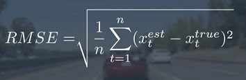
用上述公式评价估算结果与真实结果的差别,C++代码实现如下:
#include <iostream>
#include <vector>
#include "Dense"

using Eigen::MatrixXd;
using Eigen::VectorXd;
using std::cout;
using std::endl;
using std::vector;

VectorXd CalculateRMSE(const vector<VectorXd> &estimations,
    const vector<VectorXd> &ground_truth);

int main() {
  /**
   * Compute RMSE
   */
  vector<VectorXd> estimations;
  vector<VectorXd> ground_truth;

  // the input list of estimations
  VectorXd e(4);
  e << 1, 1, 0.2, 0.1;
  estimations.push_back(e);
  e << 2, 2, 0.3, 0.2;
  estimations.push_back(e);
  e << 3, 3, 0.4, 0.3;
  estimations.push_back(e);

  // the corresponding list of ground truth values
  VectorXd g(4);
  g << 1.1, 1.1, 0.3, 0.2;
  ground_truth.push_back(g);
  g << 2.1, 2.1, 0.4, 0.3;
  ground_truth.push_back(g);
  g << 3.1, 3.1, 0.5, 0.4;
  ground_truth.push_back(g);

  // call the CalculateRMSE and print out the result
  cout << CalculateRMSE(estimations, ground_truth) << endl;


  return 0;
}

VectorXd CalculateRMSE(const vector<VectorXd> &estimations,
    const vector<VectorXd> &ground_truth) {

  VectorXd rmse(4);
  rmse << 0,0,0,0;

  // check the validity of the following inputs:
  //  * the estimation vector size should not be zero
  //  * the estimation vector size should equal ground truth vector size
  if (estimations.size() != ground_truth.size()
      || estimations.size() == 0) {
    cout << "Invalid estimation or ground_truth data" << endl;
    return rmse;
  }

  // accumulate squared residuals
  for (unsigned int i=0; i < estimations.size(); ++i) {

    VectorXd residual = estimations[i] - ground_truth[i];

    // coefficient-wise multiplication
    residual = residual.array()*residual.array();
    rmse += residual;
  }

  // calculate the mean
  rmse = rmse/estimations.size();

  // calculate the squared root
  rmse = rmse.array().sqrt();

  // return the result
  return rmse;
}
输出:
0.1
0.1
0.1
0.1
25. Outro
通过上面的代码,从大的层面上,已经设计了融合系统,该系统能够融合激光和雷达传感器提供的测量值,这样我们就能估算行人的位置和速度。
后面还学习了如果实现卡尔曼滤波器,以及非线性测量模型的操作,后面还要深入学习如何处理非线性运动,如汽车的转弯等,你需要创建无损卡尔曼滤波器